4. Algebraic Loop#

4.1. Goal#

Study how PID tuning affects stability and control effort when the plant and drive are coupled through a higher-index algebraic loop.

4.2. Model Map#

System Graph

4.3. Assumptions and Scope#

No wall contact
Fixed-step co-simulation

4.4. Prerequisites and Setup#

import numpy as np
import matplotlib.pyplot as plt

from syssimx.components.fmu import FMUComponent
from syssimx.system.connection import Connection
from syssimx import System
from syssimx.viz.system_graph_visualizer import SystemGraphVisualizer

4.5. Discover FMUs#

PLATFORM = sys.platform
demo_dir_path = _repo / "demos" / "ControlledPendulum"
package_path = Path(demo_dir_path / "src/modelica/ControlledPendulum")
fmu_output_dir = Path(demo_dir_path / f"artifacts/fmus/{PLATFORM}")

fmu_paths = {}
for subdir in fmu_output_dir.iterdir():
    if subdir.is_dir():
        fmu_paths[subdir.name] = {}
        for fmu_file in subdir.glob("*.fmu"):
            fmu_paths[subdir.name][fmu_file.stem] = fmu_file
    else:
        fmu_paths[subdir.stem] = subdir

4.6. Modelica Reference Simulation#

We refer to the monolithic Modelica simulation as “Modelica” in the following. The simulation results are obtained by running the AlgebraicLoop example model in OpenModelica using the OMPython interface. The model can be found in the ControlledPendulum package.

We compare the weakly coupled system where the drive and the pendulum do not build an algebraic loop with the strongly coupled system where they do.

The weakly coupled system is obtained by replacing the DriveAdvanced component with a DriveDynamic model where there is no shared kinematic variable between the drive and the pendulum (like in the previous example).

The strongly coupled system is obtained by using the DriveAdvanced model where the drive and the pendulum share the kinematic variables theta, omega, and alpha.

4.6.1. Weakly Coupled System#

from OMPython import ModelicaSystem

ref_weak = ModelicaSystem(fileName=str(package_path / "package.mo"),
                           modelName="ControlledPendulum.Examples.NoContact.Quantization")
ref_weak.buildModel()
ref_weak.simulate(simargs={
    "stopTime": '1.0',
})
ref_sol_names = ('time', 'theta', 'theta_meas', 'u_control', 'tau')
ref_weak_sol = {name: ref_weak.getSolutions(name).flatten() for name in ref_sol_names}

4.6.2. Strongly Coupled System#

ref_strong = ModelicaSystem(fileName=str(package_path / "package.mo"),
                           modelName="ControlledPendulum.Examples.NoContact.AlgebraicLoop")
ref_strong.buildModel()
ref_strong.simulate(simargs={
    "stopTime": '1.0',
})
ref_sol_names = ('time', 'theta', 'theta_meas', 'u_control', 'tau', 'set_point.theta_ref')
ref_strong_sol = {name: ref_strong.getSolutions(name).flatten() for name in ref_sol_names}

4.6.3. Compare Weakly and Strongly Coupled Systems#

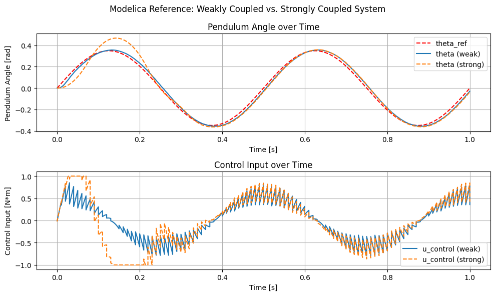
We can identify some differences between the weakly and strongly coupled systems in the trajectories of the pendulum angle theta and the control input u_control.

The strongly coupled system shows a more oscillatory behavior in both theta and u_control, which can be attributed to the algebraic loop that couples the drive and the pendulum dynamics more tightly.

The weakly coupled system, on the other hand, exhibits a smoother response due to the decoupling of the drive and pendulum dynamics.

../_images/7089c4f0036aafbcd27d436ae690c211171f65e6982b4a8323e75f1ba2ffb2f3.png

4.7. Instantiate FMU Components#

def print_parameteres(component: FMUComponent):
    print(f"Parameters of {component.name}:")
    for name, param in component.parameters.items():
        if '.' not in name and param is not None:
            print(f"  - {name}: {param}")

4.7.1. Setpoint#

setpoint = FMUComponent(name="Setpoint",
                         fmu_path=fmu_paths['Trajectories']["SetPoint"],
                         group="Reference")
print_parameteres(setpoint)

Parameters of Setpoint:
  - amplitude: 0.3490658503988659 rad
  - frequency: 2.0 Hz
  - offset: 0.0 rad
  - phase: 0.0 rad

4.7.2. PID Controller#

pid = FMUComponent(name="PID",
                   fmu_path=fmu_paths['Controllers']["PIDController"],
                   group="Controller")
print_parameteres(pid)

Parameters of PID:
  - Kd: 0.02
  - Ki: 5.0
  - Kp: 10.0
  - uMax: 1.0
  - uMin: -1.0

4.7.3. Drive#

drive = FMUComponent(name="Drive",
                     fmu_path=fmu_paths['Actuators']["DriveAdvanced"],
                     group="Actuator")

print_parameteres(drive)

Parameters of Drive:
  - I_max: 10.0 A
  - J_interface: 0.1 kg·m²
  - J_motor: 5.6×10⁻⁶ kg·m²
  - L_arm: 0.000121 H
  - R_arm: 0.151 Ohm
  - V_rated: 48.0 V
  - V_supply: 16.0 V
  - b_viscous: 0.01 m·N·s/rad
  - c: 100000.0 m·N/rad
  - d: 100.0 m·N·s/rad
  - eta: 0.85
  - gearRatio: 60.0
  - k_t: 0.03 m·N/A
  - n_0: 12916.0 1/min

4.7.4. Pendulum#

pendulum = FMUComponent(name="Pendulum",
                        fmu_path=fmu_paths['Plants']["Pendulum_cvode"],
                        group="Plant")
print_parameteres(pendulum)

Parameters of Pendulum:
  - J: 0.0442268222 kg·m²
  - L: 0.181650853 m
  - b_viscous: 0.0 m·N·s/rad
  - g: 9.81 m/s²
  - m: 1.08429606 kg
  - omega_eps: 0.001 rad/s
  - omega_start: 0.0 rad/s
  - tau_c: 0.0 m·N
  - theta_start: 0.0 rad

4.7.5. Angle Sesnsor and Decoder#

angle_sensor = FMUComponent(name="Angle Sensor",
                             fmu_path=fmu_paths['Sensors']['AngleSensor'],
                             group="Sensors")
print_parameteres(angle_sensor)

Parameters of Angle Sensor:
  - pot_range: 4.71238898038469 rad
  - r_bottom: 20000.0 Ohm
  - r_top: 80000.0 Ohm
  - samplePeriod: 0.01 s
  - theta_max: 0.45378560551852565 rad
  - theta_min: -0.45378560551852565 rad
  - v_adc: 3.0 V
  - v_pot: 5.0 V
  - nBits: 10

angle_decoder = FMUComponent(name="Angle Decoder",
                             fmu_path=fmu_paths['Sensors']['AngleDecoder'],
                             group="Signal Processing")

print_parameteres(angle_decoder)

Parameters of Angle Decoder:
  - pot_range: 4.71238898038469 rad
  - r_bottom: 20000.0 Ohm
  - r_top: 80000.0 Ohm
  - samplePeriod: 0.01 s
  - theta_max: 0.45378560551852565 rad
  - theta_min: -0.45378560551852565 rad
  - v_adc: 3.0 V
  - v_pot: 5.0 V
  - nBits: 10

4.8. Define Connections#

c1 = Connection(
    src_comp=setpoint.name,
    src_port=setpoint.output_specs["theta_ref"].name,
    dst_comp=pid.name,
    dst_port=pid.input_specs["theta_ref"].name,
)

c2 = Connection(
    src_comp=pendulum.name,
    src_port=pendulum.output_specs["theta"].name,
    dst_comp=angle_sensor.name,
    dst_port=angle_sensor.input_specs["theta"].name,
)

c3 = Connection(
    src_comp=angle_sensor.name,
    src_port=angle_sensor.output_specs["v_out"].name,
    dst_comp=angle_decoder.name,
    dst_port=angle_decoder.input_specs["v_in"].name,
)

c4 = Connection(
    src_comp=angle_decoder.name,
    src_port=angle_decoder.output_specs["theta"].name,
    dst_comp=pid.name,
    dst_port=pid.input_specs["theta_meas"].name,
)

c5 = Connection(
    src_comp=pid.name,
    src_port=pid.output_specs["u"].name,
    dst_comp=drive.name,
    dst_port=drive.input_specs["u_control"].name,
)

c6 = Connection(
    src_comp=drive.name,
    src_port=drive.output_specs["torque"].name,
    dst_comp=pendulum.name,
    dst_port=pendulum.input_specs["tau"].name,
)

c7 = Connection(
    src_comp=pendulum.name,
    src_port=pendulum.output_specs["theta"].name,
    dst_comp=drive.name,
    dst_port=drive.input_specs["phi"].name,
)

c8 = Connection(
    src_comp=pendulum.name,
    src_port=pendulum.output_specs["omega"].name,
    dst_comp=drive.name,
    dst_port=drive.input_specs["omega"].name,
)

c9 = Connection(
    src_comp=pendulum.name,
    src_port=pendulum.output_specs["alpha"].name,
    dst_comp=drive.name,
    dst_port=drive.input_specs["alpha"].name,
)

connections = [c1, c2, c3, c4, c5, c6, c7, c8, c9]
components  = [setpoint, pid, drive, pendulum, angle_decoder, angle_sensor]

4.9. Build and Initialize the System#

import logging

logging.basicConfig(
    level=logging.WARNING,  # keep third-party loggers quiet
    format="[%(module)s] %(levelname)s: %(message)s",
)
# Enable debug output for the syssimx package
logging.getLogger("syssimx").setLevel(logging.DEBUG)

system = System(name="Strongly Coupled Pendulum System")

for comp in components:
    system.add_component(comp)

for conn in connections:
    system.add_connection(conn)

system.initialize(t0=0.0)

4.10. Visualize the System Graph#

visualizer = SystemGraphVisualizer(system)
visualizer.visualize()

Warning: Could not load "C:\Users\flori\anaconda3\envs\env-312\Library\bin\gvplugin_pango.dll" - It was found, so perhaps one of its dependents was not.  Try ldd.
Warning: Could not load "C:\Users\flori\anaconda3\envs\env-312\Library\bin\gvplugin_pango.dll" - It was found, so perhaps one of its dependents was not.  Try ldd.

../_images/0d183633624d7802b2fc184437ba33bf08f3a3377e563e63c8720f756aac9f59.svg

# Silence syssimx logging for the rest of the notebook
logging.getLogger("syssimx").setLevel(logging.WARNING)

4.11. Baseline Run#

t = 0.0
dt = 0.0005
t_end = 1.0

system.run(t, t_end, dt)

history = system.get_history()

t_setpoint = history["Setpoint"][0]
theta_ref = history["Setpoint"][1]["theta_ref"]

t_pendulum = history["Pendulum"][0]
theta_pendulum = history["Pendulum"][1]["theta"]

t_decoder = history["Angle Decoder"][0]
theta_decoder = history["Angle Decoder"][1]["theta"]

t_pid = history["PID"][0]
u_control = history["PID"][1]["u"]

4.12. Plot: Basline Trajectories with Strongly Coupled System#

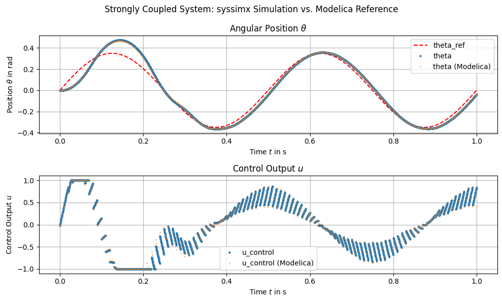
We can observe that the pendulum angle theta and the control input u_control from the syssimx simulation closely match the reference trajectories obtained from the Modelica simulation, indicating that our strongly coupled system is correctly capturing the dynamics of the original Modelica model.

../_images/51a89139d0ca291bf0f180ea0004b00db4dad09d8ada70492a7ea498eb651e48.png

4.13. Experiment Design#

We test three PID configurations and compare tracking and control effort.

4.13.1. Helper: Run a PID Case#

def run_pid_case(kp: float, ki: float, kd: float, dt: float = 0.001, t_end: float = 1.0):
    system.reset()
    pid.set_parameters(Kp=kp, Ki=ki, Kd=kd)

    system.initialize(t0=0.0)
    system.run(0.0, t_end, dt)

    history = system.get_history()

    t_ref, ref_data = history[setpoint.name]
    theta_ref = ref_data["theta_ref"]

    t_pend, pend_data = history[pendulum.name]
    theta = pend_data["theta"]

    t_drive, drive_data = history[drive.name]
    torque = drive_data["torque"]

    label = f"PID (Kp={kp}, Ki={ki}, Kd={kd})"

    return {
        "label": label,
        "t_ref": t_ref,
        "theta_ref": theta_ref,
        "t_theta": t_pend,
        "theta": theta,
        "t_torque": t_drive,
        "torque": torque,
        "kp": kp,
        "ki": ki,
        "kd": kd,
    }

4.14. PID Parameter Study#

cases = [
    run_pid_case(kp=8,  ki=8, kd=0.2),
    run_pid_case(kp=1,  ki=1, kd=0),
    run_pid_case(kp=10, ki=4, kd=0.15),
]

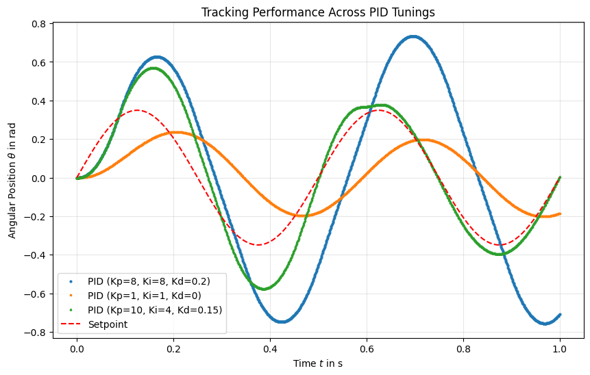
4.15. Plot: Tracking Performance#

Compare pendulum angle against the setpoint for each PID configuration.

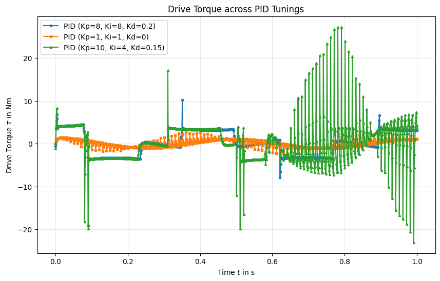
../_images/c9efe2d9587a615cf6681242076c68145bf01fb2e9e633f77dddac1d4d941d52.png

4.16. Plot: Drive Torque#

Control effort for each PID configuration.

../_images/93ef59fbb8f35d2b62e0a8db0a1f377cacca06ca4445d48945886ec4cc69b9c3.png

4.17. Summary#

We need to adapt the PID parameters to achieve good tracking performance when the drive and pendulum are coupled through an algebraic loop.
The “Medium” PID configuration shows significant oscillations and poor tracking, while the “Good” configuration achieves much better performance.
The spikes in the drive torque for the “Medium” case indicate aggressive control actions that may lead to instability, while the “Good” case shows smoother control effort.