2. FEM Pendulum: Torque Application#

In this second tutorial on the FEM implementation of the pendulum, we extend the basic model by applying an external torque at the pivot point.

Basics: We set up the basic model of a deformable pendulum without contact and external torque.
Torque Application (this tutorial): We extend the basic model by applying an external torque at the pivot point.
Contact Handling: We further extend the model by adding contact handling with a wall.

Following references were used to implement the model:

FEM pendulum torque application — Torque applied to FEM without gravitational effects.#

2.1. Overview#

This tutorial adds a torque input to the deformable 2D pendulum from Tutorial 01.

Core ideas:

Represent a desired actuator torque \(M_z^{\mathrm{drive}}(t)\) as a distributed boundary traction on the hinge edge rotation.
Choose a signed traction weight \(w(s)\) that yields zero net force but a non-zero moment (pure torque).
Implement the traction as a follower load (always normal to the current hinge edge).
Verify the implementation by applying a constant torque with gravity off and on and comparing the observed motion.

2.2. Learning Goals#

Extend the weak form of nonlinear elastodynamics by a torque-like actuation term.
Understand how a pure torque can be generated by a zero-resultant traction distribution.
Implement and motivate a follower traction (normal follows the deformed hinge edge).
Visualize and sanity-check the applied torque with and without gravity.

2.3. Prerequisites and Setup#

This notebook assumes you understand the basic setup from FEM Pendulum: Basics:

2D planar pendulum with out-of-plane thickness \(h\)
hyperelastic (Neo-Hookean) material law
hinge modeled by a mean-zero displacement constraint on the top edge rotation

Notes:

All quantities are SI.
We do not include damping or wall contact here (that is Tutorial 03).
In the documentation build, notebooks are not executed (nb_execution_mode = off).

import matplotlib.pyplot as plt
import numpy as np

from netgen.occ import *
from ngsolve import *
from ngsolve.solvers import NewtonMinimization
from ngsolve.webgui import Draw

2.4. Physical Model and Governing Equations (with torque)#

We solve nonlinear elastodynamics for the displacement field \(u(X,t)\) on the reference domain \(\Omega_0 \subset \mathbb{R}^2\).

2.4.1. Rigid-body intuition#

For a perfectly rigid pendulum with angle \(\theta(t)\), inertia \(I\) about the pivot, and center-of-mass distance \(\ell\), the equation of motion is

\[ I\,\ddot{\theta}(t) = M_z^{\mathrm{drive}}(t) - M_z^{\mathrm{grav}}(\theta), \qquad M_z^{\mathrm{grav}}(\theta) = m g \ell \sin\theta. \]

This tutorial shows how to realize the input torque \(M_z^{\mathrm{drive}}\) in a continuum FEM model.

2.4.2. Continuum elastodynamics (reference configuration)#

A standard Lagrangian form is

\[ \rho_0\,\ddot{u} = \nabla_0 \cdot P(F) + \rho_0 b \quad \text{in } \Omega_0,\qquad F = I + \nabla_0 u. \]

\(\rho_0 = \rho\,h\) is the (area) density of the 2D model with thickness \(h\).
\(P(F) = \partial W(F)/\partial F\) is the first Piola–Kirchhoff stress of the hyperelastic material.
\(b=(0,-g)\) is the body acceleration (gravity).

2.4.3. Hinge (pivot) constraint#

The top edge \(\Gamma_{\mathrm{rot}}\) is not clamped pointwise. Instead we prevent translation of that edge by enforcing the mean-zero displacement

\[ \int_{\Gamma_{\mathrm{rot}}} u\, ds = 0, \]

implemented with two Lagrange multipliers (one for \(x\), one for \(y\)). For a symmetric hinge edge whose midpoint is at the origin, this keeps the pivot fixed while allowing rotation.

2.5. From a normal traction to a pure torque#

Let \(r\) be the position vector relative to the pivot. The out-of-plane moment generated by a traction \(t\) acting on the hinge edge \(\Gamma_{\mathrm{rot}}\) is

\[ M_z = \int_{\Gamma_{\mathrm{rot}}} (r \times t)_z\, ds = \int_{\Gamma_{\mathrm{rot}}} (r_x\,t_y - r_y\,t_x)\, ds. \]

We choose a normal traction with a signed weight \(w(s)\) along the edge:

\[ t(s) = p_0\, w(s)\, n(s), \]

where \(n(s)\) is the outward unit normal and \(p_0\) is a scalar amplitude.

2.5.1. Zero net force (pure torque)#

The resultant force is

\[ F = \int_{\Gamma_{\mathrm{rot}}} t\,ds = p_0\,\int_{\Gamma_{\mathrm{rot}}} w(s)\,n(s)\,ds. \]

For a straight hinge edge with (approximately) constant normal \(n\), it is sufficient to enforce a zero-mean weight

\[ \int_{\Gamma_{\mathrm{rot}}} w(s)\, ds = 0. \]

2.5.2. Torque-to-traction conversion#

With the choice above,

\[ M_z = p_0\,\underbrace{\int_{\Gamma_{\mathrm{rot}}} w(s)\,(r \times n)_z\, ds}_{D_{\mathrm{eff}}}. \]

The factor \(D_{\mathrm{eff}}\) is a purely geometric effectiveness (an “effective lever arm”) for the chosen \(w\). We therefore set

\[ p_0 = \frac{M_z^{\mathrm{drive}}}{D_{\mathrm{eff}}}. \]

2.6. Basic Implementation#

We first mirror the setup from Tutorial 01, then add the torque application.

2.6.1. Geometry and mesh#

We reuse the same pendulum geometry as in Tutorial 01. The top edge is named rotation; its midpoint is the pivot point \((0,0)\).

# Geometry parameters
r_rod = 0.015   # rod radius in meters
r_hole = 0.03   # hole radius in meters
r_head = 0.06   # head radius in meters
l_center = 0.24 # length to center of head in meters

bar = MoveTo(-r_rod, 0).Rectangle(2 * r_rod, l_center).Face()
bar.edges.Min(Y).name = "rotation"
bar.edges.Min(Y).maxh = r_rod / 10
bar.faces.name = "bar"
bar.faces.maxh = r_rod / 2

hole = Circle((0, l_center), r_hole).Face()
hole.faces.name = "hole"
hole.edges.maxh = r_head / 20

circ = Circle((0, l_center), r_head).Face()
circ.edges.maxh = r_head / 20
circ.faces.name = "circ"
circ.faces.maxh = r_head / 5

head = circ - hole
pendulum = head + bar - hole

# Rotate so the pendulum initially points downward
pendulum = pendulum.Rotate(Axis((0.0, 0, 0), (0, 0, 1)), 180)
pendulum.name = "pendulum"

geo = OCCGeometry(pendulum, dim=2)

max_element_size = 0.03
mesh_order = 2

mesh = Mesh(geo.GenerateMesh(maxh=max_element_size))
mesh.Curve(mesh_order)

Draw(mesh)

BaseWebGuiScene

2.6.2. Material model (Neo-Hookean, plane stress)#

We reuse the compressible Neo-Hookean energy density from Tutorial 01 with the plane-stress first Lamé parameter \(\lambda^{*} = E\nu/(1-\nu^{2})\), since the pendulum is modeled as a thin plate. The 2D reduction is kept for reduced computational cost.

E = 2.1e11    # Young's modulus [Pa]
nu = 0.3      # Poisson ratio
rho = 7800    # Mass density [kg/m^3]
thickness = 0.01  # Thin plate (plane-stress assumption) [m]

# Useful reference quantities for verification
rhoA = rho * thickness

r = CF((x-0, y-0))
fem_mass = Integrate(rhoA, mesh, definedon=mesh.Materials("pendulum"))
fem_inertia = Integrate(rhoA * InnerProduct(r, r), mesh, definedon=mesh.Materials("pendulum"))

cx = Integrate(rhoA * x, mesh, definedon=mesh.Materials("pendulum")) / fem_mass
cy = Integrate(rhoA * y, mesh, definedon=mesh.Materials("pendulum")) / fem_mass
fem_l_com = np.sqrt(cx**2 + cy**2)

print(f"mass    = {fem_mass:.6f} kg")
print(f"inertia = {fem_inertia:.6f} kg*m^2")
print(f"l_com   = {fem_l_com:.6f} m")

# Plane-stress Lamé parameters (σ_zz = 0)
lam = E * nu / (1 - nu * nu)
mu = E / (2 * (1 + nu))

def C(u):
    F = Id(2) + Grad(u)
    return F.trans * F

def psi(C, lam, mu):
    return (mu / 2) * (Trace(C - Id(2)) + (2 * mu / lam) * (Det(C))**(-lam / (2 * mu)) - 1)

def PK2_neo_hookean(u, lam, mu):
    """2nd Piola-Kirchhoff stress for the Neo-Hookean model.

    S = mu * (I - det(C)^(-lam/(2*mu)) * C^{-1})
    """
    CC = C(u)
    return mu * (Id(2) - Det(CC)**(-lam / (2 * mu)) * Inv(CC))

def cauchy_stress(u, lam, mu):
    """Cauchy (true) stress: sigma = (1/J) F S F^T."""
    F = Id(2) + Grad(u)
    J = Det(F)
    S = PK2_neo_hookean(u, lam, mu)
    return (1 / J) * F * S * F.trans

def von_mises(u, lam, mu):
    """Plane-stress von Mises: sigma_vM = sqrt(sxx^2 + syy^2 - sxx*syy + 3*sxy^2)."""
    sigma = cauchy_stress(u, lam, mu)
    sxx, syy, sxy = sigma[0, 0], sigma[1, 1], sigma[0, 1]
    return sqrt(sxx * sxx + syy * syy - sxx * syy + 3 * sxy * sxy)

mass    = 1.084296 kg
inertia = 0.044227 kg*m^2
l_com   = 0.181651 m

2.6.3. FE spaces and hinge constraint#

As in Tutorial 01 we use a mixed space \(V\times Q^2\) so we can enforce

\[\int_{\Gamma_{\mathrm{rot}}} u\,ds = 0\]

via Lagrange multipliers.

V = VectorH1(mesh, order=2)
Q = NumberSpace(mesh, definedon=mesh.Boundaries("rotation"))

# Post-processing spaces on the pendulum material
S_sigma = MatrixValued(H1(mesh, order=2, definedon=mesh.Materials("pendulum")))  # Cauchy tensor
S_vm    = H1(mesh, order=2, definedon=mesh.Materials("pendulum"))                # von Mises scalar

FES = V * Q**2
(u, q), (v, p) = FES.TnT()

# State (u, multipliers)
gf_u = GridFunction(FES)
gf_v = GridFunction(FES)
gf_a = GridFunction(FES)

# Previous step (Newmark)
gf_u_old = GridFunction(FES)
gf_v_old = GridFunction(FES)
gf_a_old = GridFunction(FES)

# Stress (post-processing)
gf_sigma = GridFunction(S_sigma)  # Cauchy stress tensor
gf_vm    = GridFunction(S_vm)     # von Mises scalar

2.6.4. Residual (BilinearForm) without actuation#

We assemble the nonlinear residual using:

internal hyperelastic energy (Variation)
hinge constraint terms on rotation
inertial terms (Newmark)
gravity (toggleable via a parameter)

tau = Parameter(0.01) # time step for the implicit time integration

def build_basic_bfa(use_gravity=True):
    bfa = BilinearForm(FES)

    # Internal energy (nonlinear)
    bfa += Variation(psi(C(u), lam, mu) * dx("pendulum")).Compile()

    # Hinge constraint (mean-zero displacement on rotation edge)
    bfa += (InnerProduct(u, p) + InnerProduct(v, q)) * ds("rotation")
    
    # Newmark-style inertia term
    vel_new = 2 / tau * (u - gf_u_old.components[0]) - gf_v_old.components[0]
    acc_new = 2 / tau * (vel_new - gf_v_old.components[0]) - gf_a_old.components[0]
    bfa += rho * thickness * InnerProduct(acc_new, v) * dx("pendulum")

    # Gravity (can be switched off for verification)
    if use_gravity:
        g = 9.81
    else:
        g = 0.0
    gvec = CF((0, -g))

    bfa += -rho * thickness * InnerProduct(gvec, v) * dx("pendulum")

    return bfa

2.7. Torque Implementation in NGSolve#

The key implementation pieces are:

Compute a zero-mean weight \(w\) on the rotation edge.
Precompute \(D_{\mathrm{eff}} = \int w\,(r\times N)_z\,ds\).
Convert the desired torque \(M_z^{\mathrm{drive}}\) to a traction amplitude \(p_0 = M_z^{\mathrm{drive}}/D_{\mathrm{eff}}\).
Add the corresponding Neumann (traction) term to the residual:

\[ \int_{\Gamma_{\mathrm{rot},0}} t_{\mathrm{drive}}(u)\cdot v\,ds_0. \]

2.7.1. Follower Load#

A torque actuator at the pivot is modeled here as a pressure-like normal traction on the hinge edge rotation. If the load is meant to stay normal to that edge, then its direction must rotate together with the pendulum. This is exactly what a follower load means.

If we pick the fixed normal direction in the reference configuration, we get a traction that is not normal to the deformed edge after rotation. The produced torque then becomes angle-dependent.

Thus, we define a follower load as follows:

\[t(u) = p_0\,w\,n(u) \quad \text{on } \Gamma_{\mathrm{rot}}(u),\]

where \(n(u)\) is the outward unit normal of the deformed hinge edge.

Consequently, we need an expression for \(n(u)\) and the boundary measure scaling in reference quantities.

Let \(x = \varphi(X) = X + u(X)\) and

\[F = \nabla_X \varphi = I + \nabla_X u.\]

The surface (line) transformation provides the key identity

\[n\,J_s = \operatorname{cof}(F)\,N,\]

where

\(N\) is the outward unit normal on \(\Gamma_{\mathrm{rot},0}\),
\(n\) is the outward unit normal on the deformed edge \(\Gamma_{\mathrm{rot}}(u)\),
\(J_s\) is the surface Jacobian (line element scaling),
\(\operatorname{cof}(F)\) is the cofactor matrix (also called the adjugate), with
\[\operatorname{cof}(F) = \det(F)\,F^{-T}.\]

2.7.2. Implementation steps#

Position relative to pivot: r = CF((x-0, y-0))
Reference normal \(N\) on rotation: N_ref = specialcf.normal(2)
Deformation gradient restricted to the boundary: F = Id(2) + Grad(u).Trace()

Note: in NGSolve, .Trace() here means restrict to the boundary (it is not the matrix trace).
Cofactor (adjugate) matrix: cofF = Cof(F)
Unnormalized current normal (already includes the surface scaling):

\[nJ_s = \operatorname{cof}(F)\,N,\]

implemented as nJ_s = cofF * N_ref.
Surface Jacobian and unit normal: J_s = Norm(nJ_s) and n_cur = nJ_s / J_s.
Scalar traction amplitude: traction_amplitude = drive_parameter * weight.
Follower traction in the reference integral:

\[t_0(u) = p_0\,w\,n\,J_s,\]

implemented as applied_traction = traction_amplitude * n_cur * J_s.
Effective moment arm (torque-to-parameter map):

\[D_{\mathrm{eff}} = \int_{\Gamma_{\mathrm{rot},0}} w\,(r\times N)_z\,ds_0,\]

which lets us convert a desired torque to the scalar drive parameter.
Linear Traction Weight:

\[w_{\mathrm{lin}}(x) = \frac{x}{r_{\mathrm{rod}}} \quad \forall x \in [-r_{\mathrm{rod}}, r_{\mathrm{rod}}]\]

On the symmetric hinge edge, this weight yields a positive traction on one side of the pivot and a negative traction on the other side, resulting in a pure torque without net force.

# Reference position relative to pivot (pivot at origin)
r = CF((x - 0, y - 0))

# Reference outward normal on the rotation edge
N_ref = specialcf.normal(2)

# Traction amplitude p0 parameter
p0 = Parameter(0.0)

# Weight function (zero mean over the rotation edge)
weight = x / r_rod

# Scalar traction amplitude along the edge
traction_amplitude = p0 * weight

# Torque moment arm term (sign chosen so D_eff is typically positive)
torque_moment_arm = -(r[0] * N_ref[1] - r[1] * N_ref[0])

# Effectiveness factor: maps traction amplitude to resulting torque
D_eff = Integrate(weight * torque_moment_arm, mesh, definedon=mesh.Boundaries("rotation"))

def build_bfa(use_gravity=True, use_follower_load=True):
    # Build the basic bilinear form
    bfa = build_basic_bfa(use_gravity=use_gravity)

    if use_follower_load:
        # Follower load computation
        F = Id(2) + Grad(u).Trace()
        cofF = Cof(F)

        nJ_s = cofF * N_ref
        J_s = Norm(nJ_s)
        n_cur = nJ_s / IfPos(J_s, J_s, 1)
        
        applied_traction = traction_amplitude * n_cur * J_s
    else:
        applied_traction = traction_amplitude * N_ref

    bfa += InnerProduct(applied_traction, v) * ds("rotation")

    return bfa

2.7.3. Initial state and rigid-body proxy angle#

We initialize the pendulum by applying a rigid rotation \(\theta_0\) to the reference coordinates and setting

\[u(X,0)=R(\theta_0)X-X\]

on the pendulum material.

We also use the same rigid-body proxy as in Tutorial 01 to extract an effective angle \(\theta(t)\) from the displacement field.

def set_initial_state(theta, omega=0.0):
    c, s = np.cos(theta), np.sin(theta)

    r0 = CF((c * r[0] - s * r[1],
             s * r[0] + c * r[1]))
    u0 = CF((r0[0] - r[0],
             r0[1] - r[1]))

    gf_u.components[0].Set(u0, definedon=mesh.Materials("pendulum"))
    gf_u_old.vec[:] = gf_u.vec

    v0 = CF((-omega * r0[1], omega * r0[0]))
    gf_v.components[0].Set(v0, definedon=mesh.Materials("pendulum"))
    gf_v_old.vec[:] = gf_v.vec

    gf_a.vec[:] = 0.0
    gf_a_old.vec[:] = 0.0

def rigid_body_proxy_angle(gf_u: GridFunction) -> float:
    # Best-fit rigid rotation angle from the displacement field.

    u_sol = gf_u.components[0]

    denom = Integrate(InnerProduct(r, r), mesh, definedon=mesh.Materials("pendulum"))

    s_num = Integrate(
        r[0] * u_sol[1] - r[1] * u_sol[0],
        mesh,
        definedon=mesh.Materials("pendulum"),
    )
    c_num = Integrate(
        InnerProduct(r, r + u_sol),
        mesh,
        definedon=mesh.Materials("pendulum"),
    )

    s = s_num / denom
    c = c_num / denom

    return float(np.arctan2(s, c))

def run_simulation(dt=0.01,
                   t_end=1.0,
                   Mz=1.0,
                   theta0=0.0,
                   omega0=0.0,
                   use_gravity=True,
                   use_follower_load=True):
    bfa = build_bfa(use_gravity=use_gravity, use_follower_load=use_follower_load)

    set_initial_state(theta0, omega0)
    
    gf_u_history  = GridFunction(V, multidim=0)
    gf_vm_history = GridFunction(S_vm, multidim=0)

    p0.Set(Mz / D_eff)
    
    results = {
        't_vals': [],
        'theta_vals': [],
        'omega_vals': [],
        'torque_vals': [],
    }

    t = 0.0
    tau.Set(dt)
    n_steps = int(t_end / dt)
    for step in range(n_steps):        
        gf_u_old.vec[:] = gf_u.vec
        gf_v_old.vec[:] = gf_v.vec
        gf_a_old.vec[:] = gf_a.vec

        NewtonMinimization(
            a=bfa,
            u=gf_u,
            printing=False,
            inverse="sparsecholesky",
            maxerr=1e-6,
            maxit=20,
        )

        theta = rigid_body_proxy_angle(gf_u)

        results['t_vals'].append(t)
        results['theta_vals'].append(theta)

        gf_v.vec[:] = 2 / tau.Get() * (gf_u.vec - gf_u_old.vec) - gf_v_old.vec
        gf_a.vec[:] = 2 / tau.Get() * (gf_v.vec - gf_v_old.vec) - gf_a_old.vec

        # Post-processing: Cauchy stress tensor and plane-stress von Mises scalar
        u_cur = gf_u.components[0]
        gf_sigma.Interpolate(cauchy_stress(u_cur, lam, mu))
        gf_vm.Set(von_mises(u_cur, lam, mu))

        gf_u_history.AddMultiDimComponent(gf_u.components[0].vec)
        gf_vm_history.AddMultiDimComponent(gf_vm.vec)
        
        t += tau.Get()
        print(f"Time step {step+1}/{n_steps}, time={t:.4f} s", end="\r")
    
    results['u_history']  = gf_u_history
    results['vm_history'] = gf_vm_history

    return results

settings = {"Multidim": {"speed": 15}}

def animate(gf_hist, settings=settings):
    Draw(
        gf_hist,
        mesh,
        interpolation_multidim=True,
        deformation=gf_hist,
        animate=True,
        autoscale=True,
        settings=settings,
    )

def animate_stress(gf_sigma_hist, gf_u_hist, settings=settings):
    Draw(
        gf_sigma_hist,
        mesh,
        interpolation_multidim=True,
        deformation=gf_u_hist,
        animate=True,
        autoscale=False,
        min=0,
        max=np.max([v.FV().NumPy().max() for v in gf_sigma_hist.vecs]),
        settings=settings,
    )

Component-based animation: if you run the FEMPendulum component (not the low-level NGSolve script in this notebook), you can animate the stress history directly via fem_pendulum.animate_stress(). Ensure anim_params.animate=True to record history.

2.8. Verification#

2.8.1. Reference Rigid-body Prediction#

from scipy.integrate import solve_ivp

mass = fem_mass
length = fem_l_com
fem_inertia = fem_inertia
Mz_const = 0.2

def rigid_pendulum_dynamics(y, use_gravity=True):
    g = 9.81 if use_gravity else 0.0
    theta, omega = y
    alpha = Mz_const / fem_inertia - (fem_mass * g * length * np.sin(theta)) / fem_inertia

    return np.array([omega, alpha])

def solve_rigid_pendulum(t_span, y0, dt, use_gravity=True):
    t_eval = np.arange(t_span[0], t_span[1] + dt, dt)

    sol = solve_ivp(
        fun=lambda t, y: rigid_pendulum_dynamics(y, use_gravity=use_gravity),
        t_span=t_span,
        y0=y0,
        t_eval=t_eval,
        method='RK45',
    )

    return sol.t, sol.y[0], sol.y[1]

dt = 0.01  # Time step [s]
t_end = 1.0  # End time [s]

theta0   = 0  # Initial angle [rad]
omega0   = 0.0  # Initial angular velocity [rad/s]

2.8.2. With Follower Load#

res_1 = run_simulation(dt=dt, t_end=t_end, Mz=Mz_const,
                       theta0=theta0, omega0=omega0,
                       use_gravity=False, use_follower_load=True)
res_ref_1 = solve_rigid_pendulum(t_span=(0.0, t_end),
                                 y0=(theta0, omega0),
                                 dt=dt,
                                 use_gravity=False)
t_ref, theta_ref_1, omega_ref_1 = res_ref_1

Time step 100/100, time=1.0000 s

animate_stress(res_1['vm_history'], res_1['u_history'])

2.8.3. Without Follower Load#

res_2 = run_simulation(dt=dt, t_end=t_end, Mz=Mz_const,
                       theta0=theta0, omega0=omega0,
                       use_gravity=False, use_follower_load=False)

Time step 100/100, time=1.0000 s

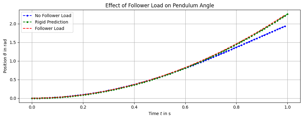
../../_images/97961e9e42e67b27c2a826947f578fd260e84076b99d6b26ba36324c0f5e2010.png

We can identify that the effect of the follower load increases as the angle increases. As the pendulum reaches \(\theta = 90 \degree\), the difference becomes more pronounced. In this position, the case No Follower Load applies a traction that is tangential to the hinge edge, producing no torque at all. The Follower Load case, however, continues to apply the full torque as desired.

2.9. Constant Torque with Gravity#

Now we repeat the same experiment with gravity enabled.

Qualitatively:

the applied torque still injects energy (no damping here), so the pendulum continues to move
gravity introduces an additional restoring moment that depends on angle

theta0 = 0
omega0 = 0

res_3 = run_simulation(dt=dt, t_end=t_end, Mz=Mz_const,
                       theta0=theta0, omega0=omega0,
                       use_gravity=True, use_follower_load=True)

res_ref_3 = solve_rigid_pendulum(t_span=(0.0, t_end),
                                 y0=(theta0, omega0),
                                 dt=dt,
                                 use_gravity=True)

Time step 100/100, time=1.0000 s

animate_stress(res_3['vm_history'], res_3['u_history'])

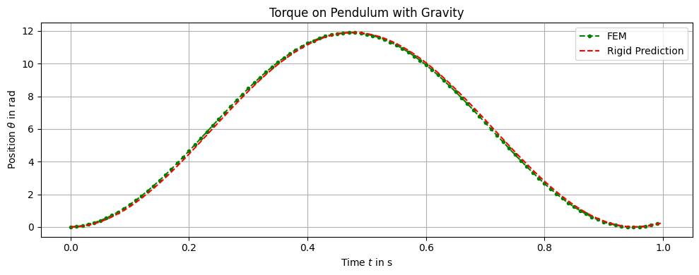
../../_images/3267a6ec11abb1584d765296a5d9b3be3b1620dbebd6d31e286c5eb353cb762c.png

We can see that the FEM simulation with follower load closely follows the rigid-body prediction.

2.10. Summary#

A desired torque can be represented by a zero-resultant traction distribution on the hinge edge.
The mapping torque \(\rightarrow\) traction uses a precomputed effectiveness factor \(D_{\mathrm{eff}}\).
To keep the traction normal to the hinge edge during large rotations, implement it as a follower load using the surface transformation \(nJ_s=\operatorname{cof}(F)N\).

Next: add wall contact and investigate how torque + contact interact (Tutorial 03).

FEM Pendulum: Torque Application

Contents