

1. OpenSim Pendulum: Basics#
In this tutorial, we build a simple rigid-body pendulum model using OpenSim and its Python API.
Basics (this tutorial): We set up a single-link pendulum with a pin joint and simulate its free swing under gravity.
Torque Application: We extend the model by applying an external torque via a
CoordinateActuator.Contact Handling: We further extend the model by adding contact geometry and forces.
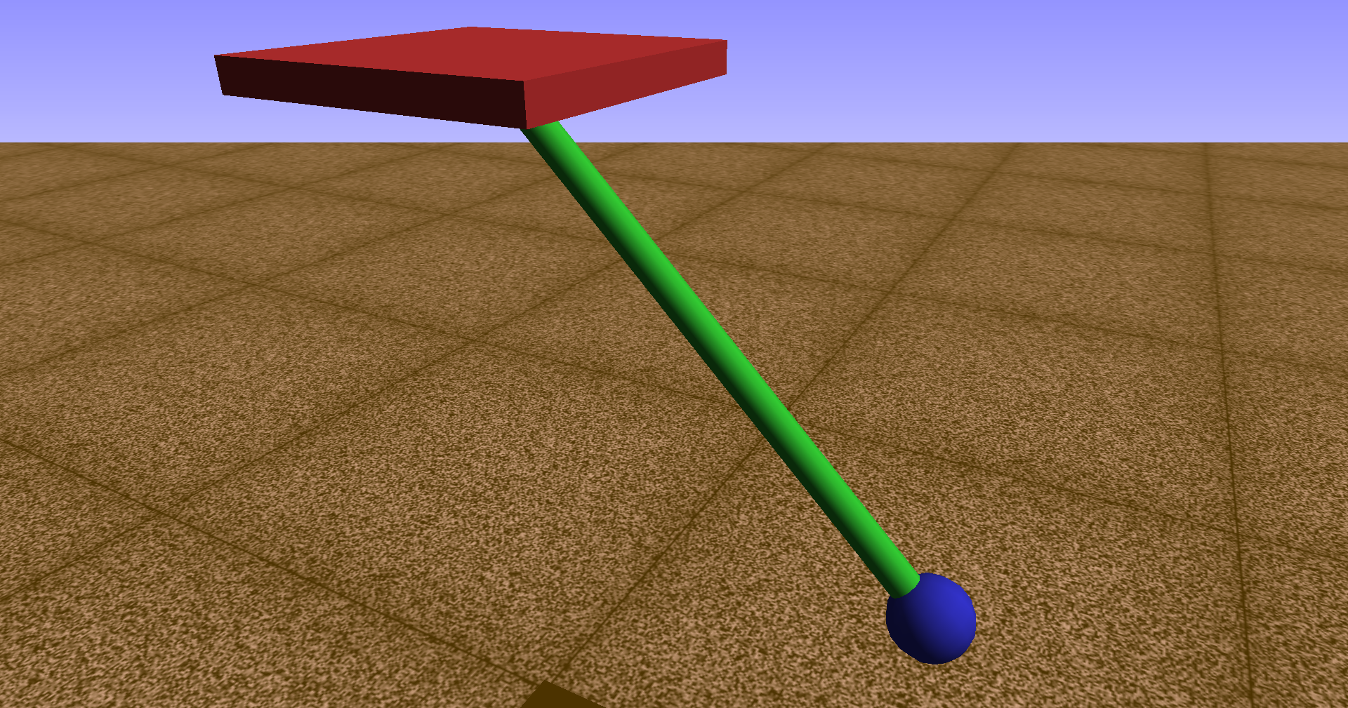
Pendulum model in the OpenSim visualizer.#
1.1. Overview#
We construct a planar pendulum from scratch using OpenSim’s building blocks:
Bodies – rigid segments with mass and inertia properties,
Joints – kinematic connections that define how bodies move relative to each other,
Geometry – visual shapes attached to bodies for visualization,
Coordinates – generalized coordinates that parameterize the joint motion,
Manager – the simulation driver that integrates the equations of motion.
This notebook focuses on the core model construction and free-swing dynamics before adding torque actuation or contact forces.
1.2. Learning Goals#
Understand the OpenSim model hierarchy:
Model → Bodies → Joints → CoordinatesCreate rigid bodies with mass properties and visualization geometry
Connect bodies using
WeldJoint(fixed) andPinJoint(1-DOF rotation)Set initial conditions via coordinate default values
Run a forward dynamics simulation using the
ManagerExtract and plot time-series results (angle, velocity, acceleration)
Perform a parameter study to compare pendulum configurations
1.3. Prerequisites and Setup#
You have installed OpenSim (version 4.x+) and its Python bindings (
opensimpackage)You have
numpyandmatplotlibavailableYou are comfortable running Jupyter Notebook cells
Background: OpenSim solves the equations of motion using the Simbody multibody dynamics engine. For a single-link pendulum with generalized coordinate \(\theta\) (the joint angle), the equation of motion is:
where \(I\) is the moment of inertia about the pivot, \(m\) is the mass, \(L\) is the distance from the pivot to the center of mass, and \(\tau\) is any applied torque. OpenSim assembles and integrates this equation (and its multi-body generalizations) automatically from the model description.
import numpy as np
import matplotlib.pyplot as plt
import opensim as osim
1.4. Physical Model#
Our pendulum consists of two bodies:
Body |
Role |
Joint to parent |
|---|---|---|
Base |
Fixed pivot point attached to ground |
|
Head |
Swinging mass at the end of a rod |
|
The PinJoint introduces a single generalized coordinate \(\theta\) that measures the rotation of the pendulum relative to the vertical. OpenSim’s convention places the rotation axis along the \(z\)-axis of the joint frames.
1.4.1. Coordinate Frames and Joint Offsets#
Each joint connects a parent frame to a child frame. The frames can be offset from the body origins:
The parent frame offset positions the joint relative to the parent body.
The child frame offset positions the joint relative to the child body.
For our pendulum, the child (head) frame is offset by the rod length \(L\) along the \(y\)-axis, so the head’s center of mass hangs at distance \(L\) below the pivot.
1.5. Model Parameters#
We define the physical parameters of the pendulum. All quantities are in SI units.
mass = 1.0         # mass of the pendulum head [kg]
r_head = 0.025     # radius of the pendulum head (visualization) [m]
length = 0.4       # length of the pendulum rod [m]
inertia_head = 0.1 # moment of inertia of the head about Z-axis [kg·m²]
g_val = 9.81       # gravitational acceleration [m/s²]
1.6. Building the OpenSim Model#
We now construct the model step by step. The general workflow is:
Create a
Modeland set gravity.Add bodies with mass, inertia, and geometry.
Connect bodies with joints.
Set default coordinate values (initial conditions).
Finalize connections.
1.6.1. Instantiate the Model and Set Gravity#
Every OpenSim model starts with a Model object. We set gravity to point in the negative \(y\)-direction, which is the standard convention.
model = osim.Model()
model.setName('Pendulum')
model.setGravity(osim.Vec3(0, -g_val, 0))
True
1.6.2. Ground Frame#
The Ground body is the immovable reference frame of the model. All other bodies are connected (directly or indirectly) to the ground through joints.
ground = model.getGround()
1.6.3. Add the Base Body (Fixed Pivot)#
The base body acts as the fixed pivot point of the pendulum. It is attached to the ground via a WeldJoint, which means it has zero degrees of freedom — it cannot move relative to the ground.
We position the base above the ground origin so the pendulum has room to swing.
Note: The base body needs a mass, but since it is welded to the ground, its mass does not affect the simulation.
base_name = "pendulum_base"
base_mass = 1.0
base_com = osim.Vec3(0, 0, 0)
base_inertia = osim.Inertia(0, 0, 0)
base = osim.Body(base_name, base_mass, base_com, base_inertia)

# Visualization: a flat brick representing the pivot support
base_geom = osim.Brick(osim.Vec3(0.1, 0.01, 0.1))
base_geom.setColor(osim.Vec3(0.8, 0.2, 0.2))
base.attachGeometry(base_geom)
model.addBody(base)
1.6.4. Weld the Base to Ground#
A WeldJoint fixes the base body at a specified position relative to the ground. We place it at a height of \(1.2 \times L\) so the pendulum can swing freely below.
ground_translation = osim.Vec3(0, 1.2 * length, 0)
ground_orientation = osim.Vec3(0, 0, 0)
base_translation = osim.Vec3(0, 0, 0)
base_orientation = osim.Vec3(0, 0, 0)

base_to_ground = osim.WeldJoint(
    "base_to_ground",
    ground,              # parent body
    ground_translation,  # position in parent frame
    ground_orientation,  # orientation in parent frame
    base,                # child body
    base_translation,    # position in child frame
    base_orientation,    # orientation in child frame
)
model.addJoint(base_to_ground)
1.6.5. Add the Pendulum Head Body#
The pendulum head is the swinging mass. We define its mass, center of mass (at the body origin), and moment of inertia about the \(z\)-axis (the rotation axis).
The Inertia constructor takes \((I_{xx}, I_{yy}, I_{zz})\) for the diagonal elements. Since the pendulum rotates about the \(z\)-axis, \(I_{zz}\) is the relevant inertia component.
head_name = "pendulum_head"
head_com = osim.Vec3(0, 0, 0)
head_inertia = osim.Inertia(0, 0, inertia_head)
head = osim.Body(head_name, mass, head_com, head_inertia)

# Visualization: a sphere representing the pendulum bob
head_geom = osim.Sphere(r_head)
head_geom.setColor(osim.Vec3(0.2, 0.2, 0.8))
head.attachGeometry(head_geom)
model.addBody(head)
1.6.6. Connect With a Pin Joint#
A PinJoint provides a single rotational degree of freedom about the \(z\)-axis of the joint frames. This is the natural choice for a planar pendulum.
Frame offsets:
The parent frame (base) is at the base body’s origin — this is the pivot location.
The child frame (head) is offset by
(0, L, 0)— meaning the head’s origin is at distance \(L\) below the joint. In OpenSim the child frame offset defines where the joint sits relative to the child body.
base_translation = osim.Vec3(0, 0, 0)
base_orientation = osim.Vec3(0, 0, 0)
head_translation = osim.Vec3(0, length, 0)
head_orientation = osim.Vec3(0, 0, 0)

head_to_base = osim.PinJoint(
    "head_to_base",
    base,              # parent body
    base_translation,  # position in parent frame
    base_orientation,  # orientation in parent frame
    head,              # child body
    head_translation,  # position in child frame
    head_orientation,  # orientation in child frame
)
model.addJoint(head_to_base)
1.6.7. Add Rod Visualization#
To visualize the rod connecting the pivot to the head, we attach a Cylinder geometry to a PhysicalOffsetFrame. This frame is fixed to the head body but offset to the midpoint of the rod.
head_of = osim.PhysicalOffsetFrame()
head_of.setName("head_of")
head_of.setParentFrame(head)
head_of.set_translation(osim.Vec3(0, length / 2, 0))

head_of_geom = osim.Cylinder(0.01, length / 2)
head_of_geom.setColor(osim.Vec3(0.2, 0.8, 0.2))
head_of.attachGeometry(head_of_geom)
head.addComponent(head_of)
1.6.8. Set Initial Conditions#
We set the default value of the pendulum coordinate \(\theta\) (angle) and its speed \(\dot{\theta}\) (angular velocity). These serve as the initial conditions for the simulation.
setDefaultValue(q0)— initial angular positionsetDefaultSpeedValue(omega0)— initial angular velocity
q0 = np.deg2rad(45)  # initial angle [rad]
omega0 = 0.0         # initial angular velocity [rad/s]

coord = head_to_base.getCoordinate()
coord.setName("theta")
coord.setDefaultValue(q0)
coord.setDefaultSpeedValue(omega0)
1.6.9. Finalize and Visualize#
Calling finalizeConnections() resolves all internal references between components. The model is then ready for simulation.
Note: The OpenSim visualizer is only available on Windows. If you are on a different platform, you can skip the visualization step and directly run the simulation.
import sys

model.finalizeConnections()

if sys.platform == 'win32':
    visualizer = osim.VisualizerUtilities()
    visualizer.showModel(model)
The visualizer window shows the pendulum in its initial configuration with \(\theta_0 = 45°\). The red brick is the fixed base, the green cylinder is the rod, and the blue sphere is the swinging mass.
1.6.10. Create .osim Model File#
To save the model for later use or to open it in the OpenSim GUI, we write it to an .osim file. This XML file contains the full model description and can be loaded by OpenSim tools.
model.printToXML("pendulum_baiscs.osim")
True
1.7. Initialize the System#
Before simulation, we initialize the system state. OpenSim uses Simbody’s realization stages to compute derived quantities (positions, velocities, forces, accelerations) on demand.
initSystem()creates an initialStateobject consistent with the model.realizeAcceleration(state)computes all quantities up to (and including) accelerations, ensuring the state is fully consistent before the simulation starts.The
Managerwraps the numerical integrator (a 5th-order Runge-Kutta-Feldberg method by default) and advances the state through time.
state = model.initSystem()
model.realizeAcceleration(state)

manager = osim.Manager(model)
manager.initialize(state)
1.8. Simulate the Free-Swinging Pendulum#
We integrate the equations of motion from \(t=0\) to \(t_\mathrm{end}\) with a reporting interval of dt. At each reporting step, we extract the coordinate value \(\theta\), speed \(\dot\theta\), and acceleration \(\ddot\theta\).
Note: The
Manager.integrate(t)call advances the internal state to time \(t\). The integrator uses adaptive step sizes internally;dthere controls how often we sample the solution, not the integration step size.
t = 0.0
dt = 0.001
t_end = 5.0

t_vals = []
theta_vals = []
omega_vals = []
alpha_vals = []

while t < t_end - 1e-8:
    state = manager.integrate(t + dt)

    theta = coord.getValue(state)
    omega = coord.getSpeedValue(state)
    model.realizeAcceleration(state)
    alpha = coord.getAccelerationValue(state)

    t_vals.append(state.getTime())
    theta_vals.append(theta)
    omega_vals.append(omega)
    alpha_vals.append(alpha)

    t = state.getTime()
1.8.1. Plot the Results#
We plot the angular position \(\theta\), angular velocity \(\dot\theta\), and angular acceleration \(\ddot\theta\) as functions of time.
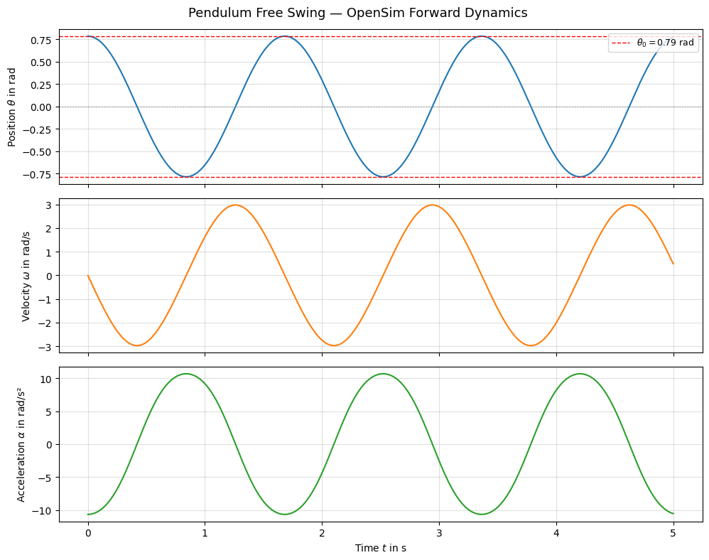
The pendulum oscillates symmetrically about the vertical (\(\theta=0\)). Since there is no damping, the amplitude remains constant. The angular velocity is zero at the turning points and maximal at the bottom, while the acceleration is proportional to \(-\sin(\theta)\).
1.8.2. Visualize the Motion#
We can replay the simulation in the OpenSim visualizer using the stored states table.
if sys.platform == 'win32':
    states_table = manager.getStatesTable()
    statesTraj = osim.StatesTrajectory.createFromStatesTable(model, states_table)
    visualizer = osim.VisualizerUtilities()
    visualizer.showMotion(model, states_table)
1.9. Conclusion#
In this tutorial we:
Built an OpenSim pendulum model using the
Body,WeldJoint, andPinJointclasses.Set initial conditions via the coordinate default values.
Ran a forward dynamics simulation using the
Managerand extracted time-series outputs.Compared different parameter configurations in a parameter study.
This model serves as the foundation for the next tutorials, where we add torque actuation and contact handling to the pendulum.