2. OpenSim Pendulum: Torque Application#

In this second tutorial on the OpenSim pendulum, we extend the basic model by applying an external torque at the pivot using a CoordinateActuator.

Basics: We set up a single-link pendulum with a pin joint and simulate its free swing under gravity.
Torque Application (this tutorial): We extend the model by applying an external torque via a CoordinateActuator.
Contact Handling: We further extend the model by adding contact geometry and forces.

2.1. Overview#

This tutorial adds a torque input to the rigid-body pendulum from Tutorial 01.

Core ideas:

Add a CoordinateActuator that applies a generalized force (torque) along the pin joint coordinate \(\theta\).
Use overrideActuation to set the torque value directly at each time step, bypassing the controller/excitation pathway.
Simulate the pendulum with a constant torque (gravity off and on) and extract time-series results.
Verify the OpenSim results against an analytical rigid-body prediction.
Compare different torque magnitudes in a parameter study.

2.2. Learning Goals#

Add a CoordinateActuator to an OpenSim model
Understand the actuation override mechanism for direct torque control
Simulate with a constant applied torque and extract kinematic outputs
Verify simulation results against a rigid-body ODE solution
Compare torque-driven motion with and without gravity

2.3. Prerequisites and Setup#

This notebook assumes you have completed Tutorial 01 — Basics and are familiar with:

Creating bodies, joints, and coordinates in OpenSim
Running forward dynamics with the Manager
Extracting coordinate values from the simulation state

Background — CoordinateActuator and Actuation Override

In OpenSim, forces are normally computed from controls (e.g., muscle excitations) through internal dynamics. For direct torque application, the CoordinateActuator class provides a simpler pathway:

A CoordinateActuator applies a scalar generalized force along a single coordinate (here, the pin joint angle \(\theta\)).
By calling overrideActuation(state, True), we bypass the normal control-to-force pipeline.
We then set the torque value directly with setOverrideActuation(state, torque_value).

This is equivalent to specifying \(\tau\) in the equation of motion:

\[I\,\ddot{\theta} = -m\,g\,L\,\sin(\theta) + \tau\]

where \(\tau\) is the value we set via setOverrideActuation.

import numpy as np
import matplotlib.pyplot as plt
import opensim as osim
from scipy.integrate import solve_ivp

2.4. Model Parameters#

We use parameters that match the FEM torque tutorial for cross-tool comparison. All quantities are in SI units.

mass = 40.0          # mass of the pendulum head [kg]
r_head = 0.05        # radius of the pendulum head (visualization) [m]
length = 0.5         # length of the pendulum rod [m]
inertia_head = 20.0  # moment of inertia of the head about Z-axis [kg·m²]
g_val = 9.81         # gravitational acceleration [m/s²]

2.5. Building the OpenSim Model#

The model construction follows Tutorial 01 (ground → base body → weld joint → head body → pin joint → rod geometry). The key addition is the CoordinateActuator.

def build_pendulum_model(use_gravity=True):
    """Build the OpenSim pendulum model with a CoordinateActuator.
    
    Returns the model, coordinate, and actuator objects.
    """
    model = osim.Model()
    model.setName('Pendulum')
    if use_gravity:
        model.setGravity(osim.Vec3(0, -g_val, 0))
    else:
        model.setGravity(osim.Vec3(0, 0, 0))

    ground = model.getGround()

    # --- Base body (fixed pivot) ---
    base = osim.Body("pendulum_base", 1.0, osim.Vec3(0), osim.Inertia(0, 0, 0))
    base_geom = osim.Brick(osim.Vec3(0.1, 0.01, 0.1))
    base_geom.setColor(osim.Vec3(0.8, 0.2, 0.2))
    base.attachGeometry(base_geom)
    model.addBody(base)

    base_to_ground = osim.WeldJoint(
        "base_to_ground",
        ground, osim.Vec3(0, 1.2 * length, 0), osim.Vec3(0),
        base, osim.Vec3(0), osim.Vec3(0),
    )
    model.addJoint(base_to_ground)

    # --- Pendulum head body ---
    head = osim.Body("pendulum_head", mass, osim.Vec3(0), osim.Inertia(0, 0, inertia_head))
    head_geom = osim.Sphere(r_head)
    head_geom.setColor(osim.Vec3(0.2, 0.2, 0.8))
    head.attachGeometry(head_geom)
    model.addBody(head)

    head_to_base = osim.PinJoint(
        "head_to_base",
        base, osim.Vec3(0), osim.Vec3(0),
        head, osim.Vec3(0, length, 0), osim.Vec3(0),
    )
    model.addJoint(head_to_base)

    # --- Rod visualization ---
    head_of = osim.PhysicalOffsetFrame()
    head_of.setName("head_of")
    head_of.setParentFrame(head)
    head_of.set_translation(osim.Vec3(0, length / 2, 0))
    head_of_geom = osim.Cylinder(r_head / 4, length / 2)
    head_of_geom.setColor(osim.Vec3(0.2, 0.8, 0.2))
    head_of.attachGeometry(head_of_geom)
    head.addComponent(head_of)

    # --- Coordinate setup ---
    coord = head_to_base.getCoordinate()
    coord.setName("theta")

    # --- CoordinateActuator (torque input) ---
    actuator = osim.CoordinateActuator()
    actuator.setName("torque")
    actuator.setCoordinate(coord)
    actuator.setOptimalForce(1)      # gain = 1 → actuation value = torque in N·m
    actuator.setMinControl(-1e6)
    actuator.setMaxControl(1e6)
    model.addForce(actuator)

    model.finalizeConnections()

    return model, coord, actuator

2.5.1. The CoordinateActuator#

A CoordinateActuator applies a generalized force along a single coordinate. Key configuration:

Method	Purpose
`setCoordinate(coord)`	Binds the actuator to the pin joint coordinate \(\theta\)
`setOptimalForce(1)`	Sets the gain to 1, so the actuation value equals the torque in N·m
`setMinControl / setMaxControl`	Sets the allowed range for torque (large bounds for unconstrained actuation)
`overrideActuation(state, True)`	Enables direct torque specification, bypassing the control pathway
`setOverrideActuation(state, τ)`	Sets the torque value \(\tau\) for the current state

Note: overrideActuation must be called after model.initSystem() because it modifies the State object.

2.6. Simulation Helper#

We encapsulate the simulation loop in a reusable function. At each reporting step, we:

Set the override actuation to the desired torque value.
Integrate to the next time point.
Realize accelerations and extract \(\theta\), \(\dot\theta\), \(\ddot\theta\).

def simulate_pendulum(model, coord, actuator, torque_func,
                      q0=0.0, omega0=0.0, dt=0.001, t_end=5.0):
    """Run a forward dynamics simulation with a time-varying torque.
    
    Parameters
    ----------
    model : osim.Model
    coord : osim.Coordinate
    actuator : osim.CoordinateActuator
    torque_func : callable
        Function torque_func(t) -> float returning the torque in N·m.
    q0 : float
        Initial angle [rad].
    omega0 : float
        Initial angular velocity [rad/s].
    dt : float
        Reporting interval [s].
    t_end : float
        End time [s].
        
    Returns
    -------
    dict with keys 'time', 'theta', 'omega', 'alpha'.
    """
    # Set initial conditions
    coord.setDefaultValue(q0)
    coord.setDefaultSpeedValue(omega0)

    state = model.initSystem()

    # Enable direct torque override
    actuator.overrideActuation(state, True)
    actuator.setOverrideActuation(state, torque_func(0.0))

    model.realizeAcceleration(state)

    manager = osim.Manager(model)
    manager.initialize(state)

    t_vals, theta_vals, omega_vals, alpha_vals = [], [], [], []

    t = 0.0
    while t < t_end - 1e-8:
        # Set torque for the upcoming integration interval
        actuator.setOverrideActuation(state, torque_func(t))

        state = manager.integrate(t + dt)
        model.realizeAcceleration(state)

        t_vals.append(state.getTime())
        theta_vals.append(coord.getValue(state))
        omega_vals.append(coord.getSpeedValue(state))
        alpha_vals.append(coord.getAccelerationValue(state))

        t = state.getTime()

    return {
        'time': np.array(t_vals),
        'theta': np.array(theta_vals),
        'omega': np.array(omega_vals),
        'alpha': np.array(alpha_vals),
    }

2.7. Analytical Reference Solution#

To verify the OpenSim results, we solve the rigid-body ODE

\[I\,\ddot{\theta} = \tau - m\,g\,L\,\sin(\theta)\]

using scipy.integrate.solve_ivp with a high-accuracy Runge-Kutta method.

def solve_rigid_pendulum(torque_val, q0, omega0, t_end, dt, use_gravity=True):
    """Solve the rigid-body pendulum ODE for verification."""
    g = g_val if use_gravity else 0.0

    def dynamics(t, y):
        theta, omega = y
        alpha = (torque_val - mass * g * length * np.sin(theta)) / (mass * length**2 + inertia_head)
        return [omega, alpha]

    t_eval = np.arange(0.0, t_end + dt, dt)
    sol = solve_ivp(dynamics, [0.0, t_end + dt], [q0, omega0],
                    t_eval=t_eval, method='RK45', rtol=1e-10, atol=1e-12)
    return sol.t, sol.y[0], sol.y[1]

2.8. Simulation Parameters#

q0 = np.deg2rad(0)    # initial angle [rad]
omega0 = 0.0           # initial angular velocity [rad/s]
dt = 0.001             # reporting interval [s]
t_end = 3.0            # end time [s]
Mz = 20.0              # constant applied torque [N·m]

2.9. Constant Torque Without Gravity#

We first disable gravity to isolate the effect of the applied torque. With \(g=0\) and constant torque \(\tau\), the analytical solution is a uniform angular acceleration:

\[\ddot\theta = \frac{\tau}{I}, \qquad \theta(t) = \theta_0 + \omega_0\,t + \frac{1}{2}\frac{\tau}{I}\,t^2.\]

This provides a clean verification of the CoordinateActuator setup.

model_ng, coord_ng, actuator_ng = build_pendulum_model(use_gravity=False)

res_ng = simulate_pendulum(
    model_ng, coord_ng, actuator_ng,
    torque_func=lambda t: Mz,
    q0=q0, omega0=omega0, dt=dt, t_end=t_end,
)

t_ref_ng, theta_ref_ng, omega_ref_ng = solve_rigid_pendulum(
    Mz, q0, omega0, t_end, dt, use_gravity=False,
)

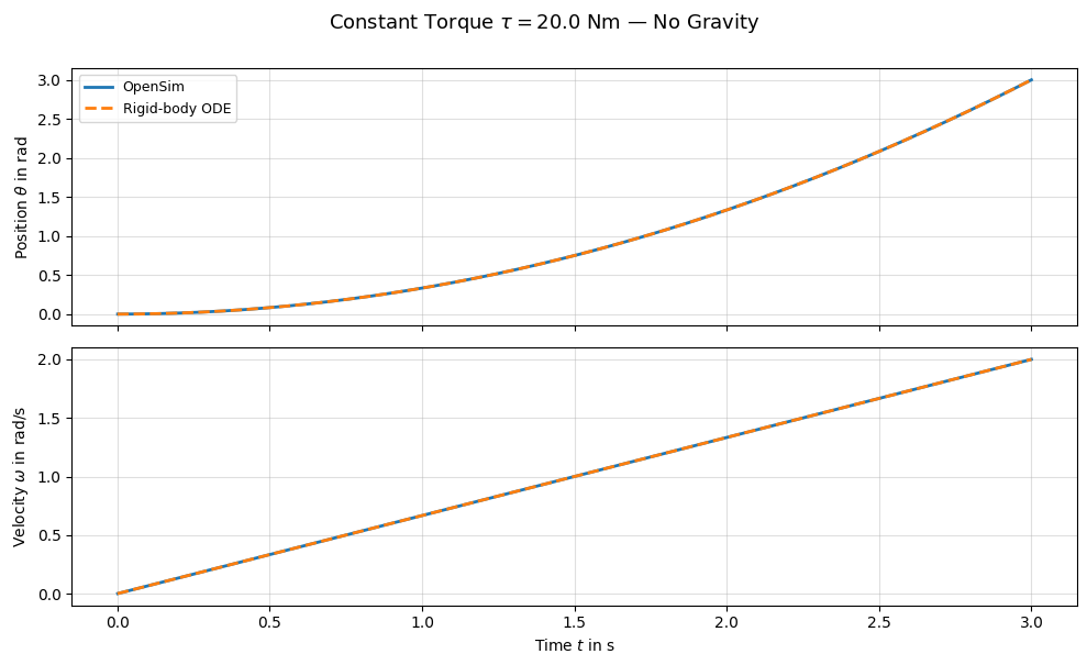
../../_images/41ebc01417008ac5f6d56b8fd4b48426b008882956cd1ec389c96a54f408fbf8.png

The OpenSim simulation matches the analytical prediction exactly. With no gravity and a constant torque, the pendulum accelerates uniformly. This confirms that the CoordinateActuator with overrideActuation correctly applies the specified torque.

2.10. Constant Torque With Gravity#

Now we enable gravity. The equation of motion becomes nonlinear due to the \(\sin(\theta)\) term:

\[I\,\ddot{\theta} = \tau - m\,g\,L\,\sin(\theta)\]

The pendulum will initially accelerate under the applied torque, but gravity provides a restoring (or opposing) moment depending on the angle.

model_g, coord_g, actuator_g = build_pendulum_model(use_gravity=True)

res_g = simulate_pendulum(
    model_g, coord_g, actuator_g,
    torque_func=lambda t: Mz,
    q0=q0, omega0=omega0, dt=dt, t_end=t_end,
)

t_ref_g, theta_ref_g, omega_ref_g = solve_rigid_pendulum(
    Mz, q0, omega0, t_end, dt, use_gravity=True,
)

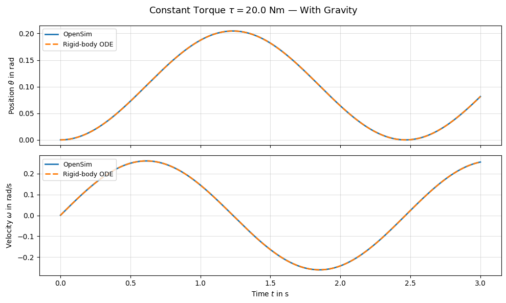
../../_images/7d837ba1226234e169bf9927bc70dd013ddb0e69e0840a6538d7077c08f72629.png

Again, the OpenSim results closely match the rigid-body ODE solution. The nonlinear interaction between the applied torque and gravity is correctly captured. Whether the torque is sufficient to drive the pendulum over the top depends on the ratio \(\tau / (m g L)\).

2.11. Comparison: Gravity On vs. Off#

We overlay both cases to highlight the effect of gravity on the torque-driven motion.

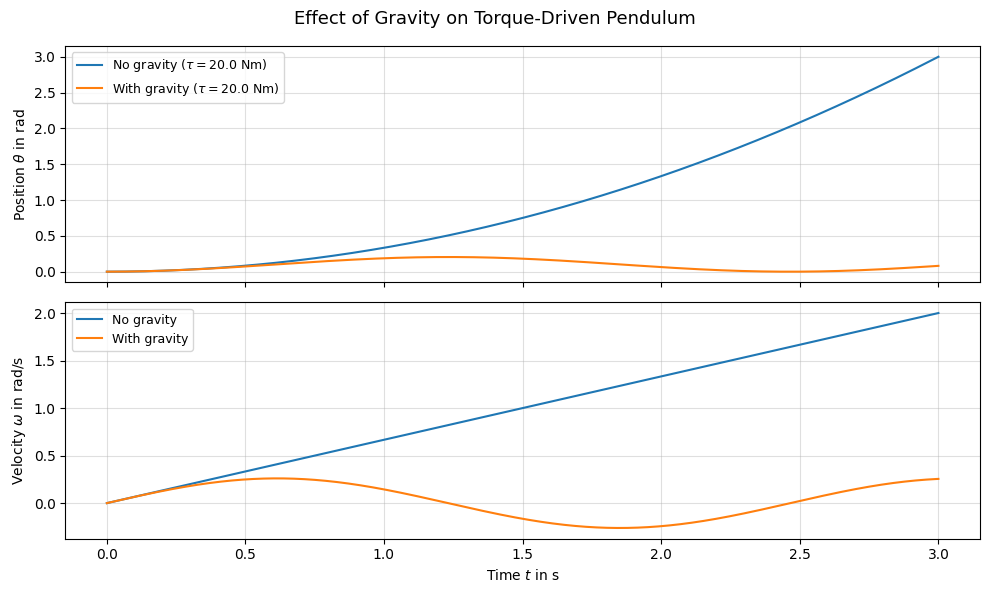
../../_images/ffa30659e0fd8ba40dfac6bbc3442ac2739c21b3a952954508e70287addec0b0.png

Without gravity, the pendulum accelerates monotonically under the constant torque. With gravity, the gravitational moment opposes or assists the motion depending on the angle, producing a more complex trajectory.

2.12. Visualize the Motion#

We can replay one of the simulations in the OpenSim visualizer.

# Rebuild and simulate for visualization (medium torque, with gravity)
model_viz, coord_viz, actuator_viz = build_pendulum_model(use_gravity=True)

coord_viz.setDefaultValue(q0)
coord_viz.setDefaultSpeedValue(omega0)
state_viz = model_viz.initSystem()
actuator_viz.overrideActuation(state_viz, True)
actuator_viz.setOverrideActuation(state_viz, Mz)
model_viz.realizeAcceleration(state_viz)

manager_viz = osim.Manager(model_viz)
manager_viz.initialize(state_viz)

t = 0.0
while t < t_end - 1e-8:
    actuator_viz.setOverrideActuation(state_viz, Mz)
    state_viz = manager_viz.integrate(t + dt)
    t = state_viz.getTime()

import sys
if sys.platform == 'win32':
    states_table = manager_viz.getStatesTable()
    visualizer = osim.VisualizerUtilities()
    visualizer.showMotion(model_viz, states_table)

2.13. Save Model#

We can write the model to an .osim file for use in the OpenSim GUI or for later reference.

model_viz.printToXML("pendulum_torque.osim")

True

2.14. Conclusion#

In this tutorial we:

Added a CoordinateActuator to apply a generalized torque along the pin joint coordinate.
Used overrideActuation to set the torque value directly at each time step, providing full control over the applied moment.
Verified the implementation against an analytical rigid-body ODE solution — both with and without gravity.

The actuation override mechanism is the key building block for co-simulation scenarios where an external controller or another simulation tool provides the torque signal at each communication step.

Next: Tutorial 03 — Contact Handling, where we add contact geometry and forces to the pendulum.

OpenSim Pendulum: Torque Application

Contents