

3. FEM Pendulum: Contact#
In this second tutorial on the FEM implementation of the pendulum, we extend the basic model by introducing a contact between the pendulum head and a wall.
Basics: We set up the basic model of a deformable pendulum without contact and external torque.
Torque Application: We extend the basic model by applying an external torque at the pivot point.
Contact Handling (this tutorial): We further extend the model by adding contact handling with a wall.
Following references were used to implement the model:
FEM pendulum contact with a wall.#
3.1. Overview#
This tutorial shows how a contact mechanism can be implemented for the pendulum. We will use the basic pendulum with torque application from the previous tutorial.
Core ideas:
We add wall as a second geometry and material to our mesh.
We define the boundary conditions and adpat the bilinear form accordingly.
We model the contact using a contact boundary between the pendulum head and the wall
We introduce a gap function which will track the gap and penetration of the contact bodies.
We use the gap function to add an energy term to the system equation which penalizes the penetration of the ball into the wall
Assumptions:
Our goal is to achive energy conservation in the system.
We neglect physical damping of the pendulum.
3.2. Learning Goals#
Extend the previous 2D planar pendulum implementation by a energy-concerving contact model
Understand how a contact can be modeled by adding an energy term to the system
Understand the effect of time step size on the energy conservation in the dynamic simulation
3.3. Prerequisites and Setup#
This notebook assumes you understand the setup from FEM Pendulum: Torque:
2D planar pendulum with out-of-plane thickness \(h\) (the 2D reduction is kept for reduced computational cost)
Plane-stress Neo-Hookean material law with \(\lambda^{*} = E\nu/(1-\nu^{2})\)
hinge modeled by a mean-zero displacement constraint on the top edge
rotationtorque actuation at the hinge via a follower load
Notes:
All quantities are SI.
We now add wall contact and study its effect on energy conservation.
import matplotlib.pyplot as plt
import numpy as np

from netgen.occ import *
from ngsolve import *
from ngsolve.solvers import NewtonMinimization
from ngsolve.webgui import Draw
3.4. Basic Implementation#
We first mirror the setup from Tutorial 01, adding the wall geometry to the mesh and defining the contact boundary.
3.4.1. Geometry and mesh#
We reuse the same pendulum geometry as in Tutorial 01. The top edge is named rotation; its midpoint is the pivot point \((0,0)\).
We add a wall geometry to the mesh, which is a rectangle at the bottom of the pendulum’s swing path. The wall has its own material properties (very stiff) and a contact boundary named contact_wall at its top edge.
# Geometry parameters
r_rod = 0.015   # rod radius in meters
r_hole = 0.03   # hole radius in meters
r_head = 0.06   # head radius in meters
l_center = 0.24 # length to center of head in meters

wall_len_x = 0.025
wall_len_y = 0.25

bar = MoveTo(-r_rod, 0).Rectangle(2 * r_rod, l_center).Face()
bar.edges.Min(Y).name = "rotation"
bar.edges.Min(Y).maxh = r_rod / 10
bar.faces.name = "bar"
bar.faces.maxh = r_rod / 2

hole = Circle((0, l_center), r_hole).Face()
hole.faces.name = "hole"
hole.edges.maxh = r_head / 20

circ = Circle((0, l_center), r_head).Face()
circ.edges.maxh = r_head / 20
circ.faces.name = "circ"
circ.faces.maxh = r_head / 5
circ.edges.name = "contact_head" # The contact surface at the head


head = circ - hole
pendulum = head + bar - hole

# Rotate so the pendulum initially points downward
pendulum = pendulum.Rotate(Axis((0.0, 0, 0), (0, 0, 1)), 180)
pendulum.name = "pendulum"

wall_pos_x = -r_head - wall_len_x
wall_pos_y = -l_center - wall_len_y / 2
wall = MoveTo(wall_pos_x, wall_pos_y).Rectangle(wall_len_x, wall_len_y).Face()
wall.faces.maxh = r_head / 5
wall.edges.Max(X).name = "contact_wall" # The contact surface at the wall
wall.edges.Max(X).maxh = r_head / 20
wall.edges.Max(Y).name = "fix" # Fixed edge
wall.edges.Min(Y).name = "fix"
wall.edges.Min(X).name = "fix"
wall.name = "wall"
geo = Compound([pendulum, wall])

geo = OCCGeometry(geo, dim=2)

max_element_size = 0.03
mesh_order = 2

mesh = Mesh(geo.GenerateMesh(maxh=max_element_size))
mesh.Curve(mesh_order)

Draw(mesh)
BaseWebGuiScene
3.4.2. Material model (Neo-Hookean, plane stress)#
We reuse the compressible Neo-Hookean energy density from Tutorial 01. Since both the pendulum and the wall are modeled as thin plates, we use the plane-stress first Lamé parameter \(\lambda^{*} = E\nu/(1-\nu^{2})\) for both bodies.
For post-processing we also expose the Cauchy stress \(\sigma = (1/J)\,F\,S\,F^{T}\) and the plane-stress von Mises equivalent stress \(\sigma_{\mathrm{vM}} = \sqrt{\sigma_{xx}^{2}+\sigma_{yy}^{2}-\sigma_{xx}\sigma_{yy}+3\sigma_{xy}^{2}}\).
def C(u):
    F = Id(2) + Grad(u)
    return F.trans * F

def psi(C, lam, mu):
    return (mu / 2) * (Trace(C - Id(2)) + (2 * mu / lam) * (Det(C))**(-lam / (2 * mu)) - 1)

def PK2_neo_hookean(u, lam, mu):
    """2nd Piola-Kirchhoff stress for the Neo-Hookean model.

    S = mu * (I - det(C)^(-lam/(2*mu)) * C^{-1})
    """
    CC = C(u)
    return mu * (Id(2) - Det(CC)**(-lam / (2 * mu)) * Inv(CC))

def cauchy_stress(u, lam, mu):
    """Cauchy (true) stress: sigma = (1/J) F S F^T."""
    F = Id(2) + Grad(u)
    J = Det(F)
    S = PK2_neo_hookean(u, lam, mu)
    return (1 / J) * F * S * F.trans

def von_mises(u, lam, mu):
    """Plane-stress von Mises: sigma_vM = sqrt(sxx^2 + syy^2 - sxx*syy + 3*sxy^2)."""
    sigma = cauchy_stress(u, lam, mu)
    sxx, syy, sxy = sigma[0, 0], sigma[1, 1], sigma[0, 1]
    return sqrt(sxx * sxx + syy * syy - sxx * syy + 3 * sxy * sxy)
def lam_mu_from_E_nu(E, nu):
    # Plane-stress Lamé parameters (σ_zz = 0)
    lam = E * nu / (1 - nu * nu)
    mu = E / (2 * (1 + nu))
    return lam, mu
3.4.3. FE spaces and hinge constraint#
As in Tutorial 01 we use a mixed space \(V\times Q^2\) so we can enforce
via Lagrange multipliers.
V = VectorH1(mesh, order=2, dirichlet="fix") # Dirichlet on fixed wall edge
Q = NumberSpace(mesh, definedon=mesh.Boundaries("rotation"))

# Post-processing spaces (defined on both materials; sampled on pendulum only)
S_sigma = MatrixValued(H1(mesh, order=2))  # Cauchy tensor
S_vm    = H1(mesh, order=2)                # von Mises scalar

FES = V * Q**2
(u, q), (v, p) = FES.TnT()

# State (u, multipliers)
gf_u = GridFunction(FES)
gf_v = GridFunction(FES)
gf_a = GridFunction(FES)

# Previous step (Newmark)
gf_u_old = GridFunction(FES)
gf_v_old = GridFunction(FES)
gf_a_old = GridFunction(FES)

# Stress (post-processing)
gf_sigma = GridFunction(S_sigma)  # Cauchy stress tensor
gf_vm    = GridFunction(S_vm)     # von Mises scalar
3.4.4. Basic Bilinear Form with Torque#
tau = Parameter(0.01) # time step for the implicit time integration

def build_basic_bfa(config, use_gravity=True):
    bfa = BilinearForm(FES)

    lam_pend, mu_pend = lam_mu_from_E_nu(config['pendulum']['E'], config['pendulum']['nu'])
    lam_wall, mu_wall = lam_mu_from_E_nu(config['wall']['E'], config['wall']['nu'])

    rhoA_pend = config['pendulum']['rho'] * config['pendulum']['thickness']
    rhoA_wall = config['wall']['rho'] * config['wall']['thickness']

    # Internal energy (nonlinear)
    bfa += Variation(psi(C(u), lam_pend, mu_pend) * dx("pendulum")).Compile()
    bfa += Variation(psi(C(u), lam_wall, mu_wall) * dx("wall")).Compile()

    # Hinge constraint (mean-zero displacement on rotation edge)
    bfa += (InnerProduct(u, p) + InnerProduct(v, q)) * ds("rotation")

    # Newmark-style inertia term
    vel_new = 2 / tau * (u - gf_u_old.components[0]) - gf_v_old.components[0]
    acc_new = 2 / tau * (vel_new - gf_v_old.components[0]) - gf_a_old.components[0]
    bfa += rhoA_pend * InnerProduct(acc_new, v) * dx("pendulum")
    bfa += rhoA_wall * InnerProduct(acc_new, v) * dx("wall")

    # Gravity (can be switched off for verification)
    if use_gravity:
        g = 9.81
    else:
        g = 0.0
    gvec = CF((0, -g))
    bfa += -rhoA_pend * InnerProduct(gvec, v) * dx("pendulum")
    bfa += -rhoA_wall * InnerProduct(gvec, v) * dx("wall")

    return bfa
# Reference position relative to pivot (pivot at origin)
r = CF((x - 0, y - 0))

# Reference outward normal on the rotation edge
N_ref = specialcf.normal(2)

# Traction amplitude p0 parameter
p0 = Parameter(0.0)

# Weight function (zero mean over the rotation edge)
weight = x / r_rod

# Scalar traction amplitude along the edge
traction_amplitude = p0 * weight

# Torque moment arm term (sign chosen so D_eff is typically positive)
torque_moment_arm = -(r[0] * N_ref[1] - r[1] * N_ref[0])

# Effectiveness factor: maps traction amplitude to resulting torque
D_eff = Integrate(weight * torque_moment_arm, mesh, definedon=mesh.Boundaries("rotation"))
def add_torque_to_bfa(bfa):
    # Follower load computation
    F = Id(2) + Grad(u).Trace()
    cofF = Cof(F)

    nJ_s = cofF * N_ref
    J_s = Norm(nJ_s)
    n_cur = nJ_s / IfPos(J_s, J_s, 1)

    applied_traction = traction_amplitude * n_cur * J_s

    bfa += InnerProduct(applied_traction, v) * ds("rotation")

    return bfa
3.5. Contact Setup#
We extend the bilinear form from Tutorial 02 by adding a contact boundary and the corresponding energy term.
3.5.1. 3.1 Contact Boundary#
cb = ContactBoundary(mesh.Boundaries("contact_wall"), mesh.Boundaries("contact_pendulum"))
We define a contact boundary cb between the contact edge of the wall and the contact edge of the pendulum head.
The contact_wall boundary acts as the master surface, while the contact_pendulum boundary acts as the slave surface.
To setup an incremental gao formulation, we define the following variables:
X_M: Master surface reference coordinates (undeformed configuration)X_S: Slave surface reference coordinates (undeformed configuration)n_S: Inverted normal vector of the slave surface (points outwards from the master/wall surface)Gap function
cf: scalar valued coefficient function that depends on the normal gap between master and slave surface
3.5.1.1. Incremental Gap Formulation#
We are using the incremental gap formulation introduced in Contact Problems - NGS Docu Interactive Tutorial.
This formulation considers the displacement changes between time steps, rather than the absolute displacements. This is particularly useful in dynamic simulations where the contact conditions may change frequently.
The following expression defines the gap formulation:
where
\(u_M\), \(u_S\): current displacements at master and slave
\(u_{old,M}\), \(u_{old,S}\): displacements at previous time step at master and slave
\(X_M\), \(X_S\): reference coordinates of master and slave
\(n_S\): normal vector at slave surface
3.5.1.2. Contact Energy Term#
The gap function cf computes the distance between the master and slave surfaces in normal direction.
A penalty energy term kn * cf * cf is added that increases quadratically as penetration depth increases
The conditional IfPos(cf, penalty_energy, 0) ensures that the penalty term is only active when the gap function indicates penetration (i.e., cf >0)
If a nearly rigid contact is desired, the penalty parameter k_n must be sufficiently large to prevent significant penetration
3.5.1.3. Contact Update#
cb.Update(uold, bfmstar, intorder=5, maxdist=0.01, both_sides=False)
The contact is updated within each time step contact.Update() before solving the variational problem with MinimizeNewton()
The displacement grid function uold is copied to an internal grid function, and the the defined contact energy contributions are evaluated and inserted into the bilinear form bfmstar
The argument intorder defines the integration order for the master side quadrature and valuation of the contact energy.
The argument maxdist defines maximum search distance (default: \(2 \cdot \max{d_\text{element}}\)) for finding contact partners on the master surface.
def initialize_contact(kn=1e10):
    """
    Initialize contact boundary conditions using penalty method and incremental gap function.
    """
    master = mesh.Boundaries("contact_wall")
    slave = mesh.Boundaries("contact_head")
    contact = ContactBoundary(master, slave)

    u_old = gf_u_old.components[0]

    X_M = CoefficientFunction((x, y))
    X_S = X_M.Other()
    n_S = -specialcf.normal(2).Other()

    increment_master = X_M + u - u_old
    increment_slave = X_S + u.Other() - u_old.Other()
    cf = (increment_master - increment_slave) * n_S

    penalty_energy = kn * cf * cf
    contact.AddEnergy(IfPos(cf, penalty_energy, 0), deformed=True)
    return contact
The function get_contact_gap_distnce computes the minimum normal gap between two boundary elements.
Updates the contact state using the current displacement field (
gf_u.components[0]). This refreshes the contact data so the gap and surface normal are consistent with the current deformation.Builds the normal gap field by projecting the vector gap onto the contact normal:
\[g_n(x) = \mathbf{g}(x) \cdot \mathbf{n}(x)\]This yields a scalar gap in normal direction.Samples the normal gap on the boundary: it loops over all boundary elements, selects those with
el.mat == "contact_wall", and evaluates the normal gap at quadrature (integration) points on each selected element.Returns the minimum value found across all sampled points.
Interpretation of the result:
min_gap > 0→ surfaces are separated (a positive clearance exists everywhere sampled).min_gap < 0→ penetration occurs somewhere on the boundary (constraint violation or active contact, depending on the formulation).
Practical notes:
The minimum gap is approximated by evaluations at integration points (order 6 in this function). Higher integration order can improve accuracy at the cost of performance.
If no valid evaluations are obtained (e.g., evaluation fails at all points), the function returns
0.0as a fallback.
def get_contact_gap_distance(contact, bfa, gf_u, mesh):
    """
    Compute the minimum gap distance at the contact interface.
    Returns:
        float: Minimum gap distance
    """
    contact.Update(gf_u.components[0], bfa, intorder=10, maxdist=0.5)
    gap_vec_master = contact.gap
    n_master = contact.normal
    gap_n_master = InnerProduct(gap_vec_master, n_master)
    gap_values = []
    for el in mesh.Elements(BND):
        if el.mat == "contact_wall":
            trafo = mesh.GetTrafo(el)
            ir = IntegrationRule(el.type, order=6)
            for ip in ir:
                mapped_ip = trafo(ip)
                try:
                    gap_val = gap_n_master(mapped_ip)
                    gap_values.append(gap_val)
                except:
                    continue
    min_gap = min(gap_values) if gap_values else 0.0
    return min_gap
The following helper function are mirrored from the previous tutorials.
def set_initial_state(theta, omega=0.0):
    c, s = np.cos(theta), np.sin(theta)

    r0 = CF((c * r[0] - s * r[1],
             s * r[0] + c * r[1]))
    u0 = CF((r0[0] - r[0],
             r0[1] - r[1]))

    gf_u.components[0].Set(u0, definedon=mesh.Materials("pendulum"))
    gf_u_old.vec[:] = gf_u.vec

    v0 = CF((-omega * r0[1], omega * r0[0]))
    gf_v.components[0].Set(v0, definedon=mesh.Materials("pendulum"))
    gf_v_old.vec[:] = gf_v.vec

    gf_a.vec[:] = 0.0
    gf_a_old.vec[:] = 0.0
def rigid_body_proxy_angle(gf_u: GridFunction) -> float:
    # Best-fit rigid rotation angle from the displacement field.

    u_sol = gf_u.components[0]

    denom = Integrate(InnerProduct(r, r), mesh, definedon=mesh.Materials("pendulum"))

    s_num = Integrate(
        r[0] * u_sol[1] - r[1] * u_sol[0],
        mesh,
        definedon=mesh.Materials("pendulum"),
    )
    c_num = Integrate(
        InnerProduct(r, r + u_sol),
        mesh,
        definedon=mesh.Materials("pendulum"),
    )

    s = s_num / denom
    c = c_num / denom

    return float(np.arctan2(s, c))
settings = {"Multidim": {"speed": 15}}

def animate(results, settings=settings):
    Draw(
        results["vm_history"],
        mesh,
        interpolation_multidim=True,
        deformation=results["u_history"],
        animate=True,
        autoscale=False,
        min=np.min(results["vm_history"].vecs),
        max=np.max(results["vm_history"].vecs),
        settings=settings,
    )
3.6. Define Material Configurations#
We are defining two material configurations, one for a stiff pendulum and one for a compliant pendulum. The wall is modeled in both cases as a very stiff material.
stiff_config = {
    'pendulum': {
        'E': 2.1e11,
        'nu': 0.3,
        'rho': 7850,
        'thickness': 0.01,  # thin plate (plane-stress assumption)
    },
    'wall': {
        'E': 2.1e11,
        'nu': 0.3,
        'rho': 7850,
        'thickness': 0.01,  # thin plate (plane-stress assumption)
    },
    'kn': 1e10
}

compliant_config = {
    'pendulum': {
        'E': 1e6,
        'nu': 0.45,
        'rho': 1000,
        'thickness': 0.01,  # thin plate (plane-stress assumption)
    },
    'wall': {
        'E': 2.1e11,
        'nu': 0.3,
        'rho': 7850,
        'thickness': 0.01,  # thin plate (plane-stress assumption)
    },
    "kn": 2.5e7

}
bfa = build_basic_bfa(config=stiff_config, use_gravity=True)
bfa = add_torque_to_bfa(bfa)
contact = initialize_contact(kn=stiff_config["kn"])
3.6.1. Positive Gap Distance - No Contact#
By setting the initial position of the pendulum head such that it does not penetrate the wall, we can observe a positive gap distance.
theta0 = np.deg2rad(10) # Initial angle in degrees
set_initial_state(theta0)
scene = Draw(gf_u.components[0], mesh, deformation=gf_u.components[0])
gap = get_contact_gap_distance(contact, bfa, gf_u, mesh)
print(f"Initial contact gap distance: {gap:.6e} m")
Initial contact gap distance: 4.167561e-02 m
3.6.2. Negative Gap Distance - Penetration#
By setting the initial position of the pendulum head such that it penetrates the wall, we can observe a negative gap distance.
theta0 = np.deg2rad(-2) # Initial angle in degrees
set_initial_state(theta0)
scene = Draw(gf_u.components[0], mesh, deformation=gf_u.components[0])
gap = get_contact_gap_distance(contact, bfa, gf_u, mesh)
print(f"Initial contact gap distance: {gap:.6e} m")
Initial contact gap distance: -8.374371e-03 m
We define the following helper function to run different simulations with different initial conditions and material parameters.
def run_simulation(
    dt = 0.001,
    t_end = 1.0,
    theta0 = np.deg2rad(20),
    config=stiff_config,
    use_adaptive_time_stepping=False):

    lam_pend, mu_pend = lam_mu_from_E_nu(config['pendulum']['E'], config['pendulum']['nu'])
    lam_wall, mu_wall = lam_mu_from_E_nu(config['wall']['E'], config['wall']['nu'])

    bfa = build_basic_bfa(config=config, use_gravity=True)
    bfa = add_torque_to_bfa(bfa)
    contact = initialize_contact(kn=config["kn"])

    set_initial_state(theta0)

    gf_u_history  = GridFunction(V, multidim=0)
    gf_vm_history = GridFunction(S_vm, multidim=0)

    results = {
        'time': np.ndarray([]),
        'theta': np.ndarray([]),
        'gap': np.ndarray([]),
    }

    t = 0.0
    dt_initial = dt
    tau.Set(dt)
    with TaskManager():
        while t < t_end - 1e-8:
            dt = min(t_end - t, dt_initial)
            tau.Set(dt)

            gf_u_old.vec[:] = gf_u.vec
            gf_v_old.vec[:] = gf_v.vec
            gf_a_old.vec[:] = gf_a.vec

            contact.Update(gf_u.components[0], bfa, intorder=10, maxdist=1)

            if use_adaptive_time_stepping:
                gap = get_contact_gap_distance(contact, bfa, gf_u, mesh)
                if    gap < 1e-3:  tau.Set(1e-4)
                elif  gap < 5e-3:  tau.Set(5e-4)
                elif  gap < 1e-2:  tau.Set(1e-3)

                else: tau.Set(dt)

            NewtonMinimization(
                a=bfa,
                u=gf_u,
                printing=False,
                inverse="sparsecholesky",
                maxerr=1e-6,
                maxit=20,
            )

            gf_v.vec[:] = 2 / tau.Get() * (gf_u.vec - gf_u_old.vec) - gf_v_old.vec
            gf_a.vec[:] = 2 / tau.Get() * (gf_v.vec - gf_v_old.vec) - gf_a_old.vec

            # Post-processing: Cauchy stress tensor and plane-stress von Mises scalar
            u_cur = gf_u.components[0]
            gf_sigma.Interpolate(cauchy_stress(u_cur, lam_pend, mu_pend), definedon=mesh.Materials("pendulum"))
            gf_vm.Set(von_mises(u_cur, lam_pend, mu_pend), definedon=mesh.Materials("pendulum"))

            gf_u_history.AddMultiDimComponent(gf_u.components[0].vec)
            gf_vm_history.AddMultiDimComponent(gf_vm.vec)

            t += tau.Get()
            gap = get_contact_gap_distance(contact, bfa, gf_u, mesh)
            theta = rigid_body_proxy_angle(gf_u)
            print(f"t = {t:.5f} / {t_end} s, \t dt = {tau.Get():.5f} s, \t gap = {gap:.5f} m", end="\r")

            results['time'] = np.append(results['time'], t)
            results['gap'] = np.append(results['gap'], gap)
            results['theta'] = np.append(results['theta'], theta)

    results['u_history']  = gf_u_history
    results['vm_history'] = gf_vm_history

    return results
results_non_adaptive = run_simulation(config=stiff_config,
                                      use_adaptive_time_stepping=False)
t = 1.00000 / 1.0 s, dt = 0.00100 s, gap = 0.12856 mm
results_adaptive = run_simulation(config=stiff_config,
                                  use_adaptive_time_stepping=True)
t = 1.00000 / 1.0 s, dt = 0.00090 s, gap = 0.08034 mm
#animate(results_adaptive)
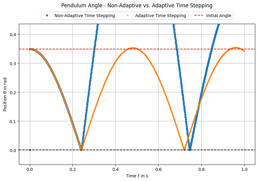
We can see that for non-adative time stepping, the energy is not conserved, since the the pendulum reaches a greater maximum angle after contact than before.
This means, that the energy which is added by the contact model (due to penetration) is too high. A reason for this is the time discretization error, which leads to an overestimation of the penetration depth when using large time steps.
When using adaptive time stepping, the time step is reduced around the contact event, leading to a more accurate estimation of the penetration depth and thus better energy conservation.
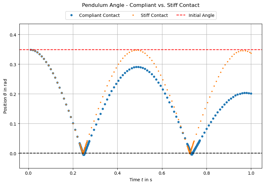
3.7. Compliant Pendulum Contact#
# res_compliant = run_simulation(config=compliant_config,
#                                use_adaptive_time_stepping=True)
#animate(res_compliant)
We can identify a minimal penetration of the compliant pendulum into the wall, which is expected due to the lower stiffness of the pendulum material. Further, we can see that the pendulum shows a elastic deformation at the contact point, which is also expected due to the compliant material properties.
The less stiff the pendulum material is, the less appropriate is the rigid body approximation for the pendulum angle. It can be observed that the pendulum starts rod and head starts to oscillate.
3.8. Conclusion#
In this tutorial section, we have extended the basic FEM pendulum model by introducing a contact mechanism with a wall. We have seen how to define a contact boundary, implement an incremental gap formulation, and add a penalty energy term to model the contact interaction.
Together, with the previous tutorials, we have now a complete FEM model of a 2D planar pendulum with torque application and contact handling.
Now, you can inspect the FEMPendulum (see demos/ControlledPendulum/src/master_pendulum/components/fem/fem_pendulum.py) class to see how all these components come together in a single simulation model corresponding to the CoSimComponent interface of the syssimx framework.