

2. Baseline System Model#
2.1. Goal#
Build the simplest closed-loop controlled pendulum using FMU components and compare it against a monolithic Modelica reference simulation.
2.2. Model Map#

2.3. Assumptions and Scope#
No sensors/decoders and no contact
Fixed-step co-simulation; reference uses variable-step DASSL
2.4. Prerequisites and Setup#
import numpy as np
import matplotlib.pyplot as plt

from demos.ControlledPendulum.src.master_pendulum import MasterPendulum
import demos.ControlledPendulum.src.master_pendulum.components.fem.pendulum_config as config

from syssimx import FMUComponent, Connection, System, SystemGraphVisualizer
2.5. Discover FMUs#
PLATFORM = sys.platform
demo_dir_path = _repo / "demos" / "ControlledPendulum"
package_path = Path(demo_dir_path / "src/modelica/ControlledPendulum")
fmu_output_dir = Path(demo_dir_path / f"artifacts/fmus/{PLATFORM}")

fmu_paths = {}
for subdir in fmu_output_dir.iterdir():
    if subdir.is_dir():
        fmu_paths[subdir.name] = {}
        for fmu_file in subdir.glob("*.fmu"):
            fmu_paths[subdir.name][fmu_file.stem] = fmu_file
        for subsubdir in subdir.iterdir():
            fmu_paths[subdir.name][subsubdir.name] = {}
            if subsubdir.is_dir():
                fmu_paths[subdir.name][subsubdir.name] = {}
                for fmu_file in subsubdir.glob("*.fmu"):
                    fmu_paths[subdir.name][subsubdir.name][fmu_file.stem] = fmu_file
    else:
        fmu_paths[subdir.stem] = subdir
2.6. Modelica Reference Simulation#
We refer to the monolithic Modelica simulation as “Modelica” in the following. The simulation results are obtained by running the Baseline example model in OpenModelica using the OMPython interface. The model can be found in the ControlledPendulum package
from OMPython import ModelicaSystem
reference = ModelicaSystem(fileName=str(package_path / "package.mo"),
                           modelName="ControlledPendulum.Examples.NoContact.Baseline")
reference.getSimulationOptions()
{'startTime': '0',
 'stopTime': '2',
 'stepSize': '0.001',
 'tolerance': '1e-06',
 'solver': 'dassl',
 'outputFormat': 'mat'}
reference.setSimulationOptions(simOptions={
    "stopTime": '1.0',
})
reference.buildModel()

reference.getSimulationOptions()
{'startTime': '0',
 'stopTime': '2',
 'stepSize': '0.001',
 'tolerance': '1e-06',
 'solver': 'dassl',
 'outputFormat': 'mat'}
reference.simulate(simargs={
    "stopTime": '1.0',
})
ref_sol_names = ('time', 'theta', 'omega', 'u_control')
ref_sol = {name: reference.getSolutions(name).flatten() for name in ref_sol_names}
2.7. Instantiate FMU Components#
def print_parameteres(component: FMUComponent):
    print(f"Parameters of {component.name}:")
    for name, param in component.parameters.items():
        if '.' not in name and param is not None:
            print(f"  - {name}: {param}")
2.7.1. Setpoint#
setpoint = FMUComponent(name="Setpoint",
                         fmu_path=fmu_paths['Trajectories']["SetPoint"],
                         group="Reference")
print_parameteres(setpoint)
Parameters of Setpoint:
  - amplitude: 0.3490658503988659 rad
  - frequency: 2.0 Hz
  - offset: 0.0 rad
  - phase: 0.0 rad
2.7.2. PID Controller#
pid = FMUComponent(name="PID",
                   fmu_path=fmu_paths['Controllers']["PIDController"],
                   group="Controller")
print_parameteres(pid)
Parameters of PID:
  - Kd: 0.02
  - Ki: 5.0
  - Kp: 10.0
  - uMax: 1.0
  - uMin: -1.0
2.7.3. Drive#
drive = FMUComponent(name="Drive",
                     fmu_path=fmu_paths['Actuators']["DriveDynamic"],
                     group="Actuator")
print_parameteres(drive)
Parameters of Drive:
  - I_max: 10.0 A
  - L_arm: 0.000121 H
  - R_arm: 0.151 Ohm
  - V_rated: 48.0 V
  - V_supply: 16.0 V
  - eta: 0.85
  - gearRatio: 60.0
  - k_t: 0.03 m·N/A
  - n_0: 12916.0 1/min
2.7.4. Pendulum#
pendulum = FMUComponent(name="Pendulum",
                        fmu_path=fmu_paths['Plants']["Pendulum_cvode"],
                        group="Plant")
print_parameteres(pendulum)
Parameters of Pendulum:
  - J: 0.0442268222 kg·m²
  - L: 0.181650853 m
  - b_viscous: 0.0 m·N·s/rad
  - g: 9.81 m/s²
  - m: 1.08429606 kg
  - omega_eps: 0.001 rad/s
  - omega_start: 0.0 rad/s
  - tau_c: 0.0 m·N
  - theta_start: 0.0 rad
2.8. Define Connections#
c1 = Connection(
    src_comp=setpoint.name,
    src_port=setpoint.output_specs["theta_ref"].name,
    dst_comp=pid.name,
    dst_port=pid.input_specs["theta_ref"].name,
)

c2 = Connection(
    src_comp=pendulum.name,
    src_port=pendulum.output_specs["theta"].name,
    dst_comp=pid.name,
    dst_port=pid.input_specs["theta_meas"].name,
)

c3 = Connection(
    src_comp=pid.name,
    src_port=pid.output_specs["u"].name,
    dst_comp=drive.name,
    dst_port=drive.input_specs["u_control"].name,
)

c4 = Connection(
    src_comp=drive.name,
    src_port=drive.output_specs["torque"].name,
    dst_comp=pendulum.name,
    dst_port=pendulum.input_specs["tau"].name,
)

c5 = Connection(
    src_comp=pendulum.name,
    src_port=pendulum.output_specs["omega"].name,
    dst_comp=drive.name,
    dst_port=drive.input_specs["omega"].name,
)

connections = [c1, c2, c3, c4, c5]
components  = [setpoint, pid, drive, pendulum]
2.9. Build and Initialize the System#
2.10. Visualize the System Graph#
visualizer = SystemGraphVisualizer(system)
visualizer.visualize()
Warning: Could not load "C:\Users\flori\anaconda3\envs\env-312\Library\bin\gvplugin_pango.dll" - It was found, so perhaps one of its dependents was not.  Try ldd.
Warning: Could not load "C:\Users\flori\anaconda3\envs\env-312\Library\bin\gvplugin_pango.dll" - It was found, so perhaps one of its dependents was not.  Try ldd.

2.11. Run Simulation#
t = 0.0
dt = 0.01
t_end = 1.0
dt_vals = (0.015, 0.01, 0.005)

histories = {}

for dt in dt_vals:
    system.reset()
    system.initialize(t0=0.0)
    system.run(t0=0.0, tf=t_end, dt=dt)
    histories[f'{dt:.3f}s'] = system.get_history()
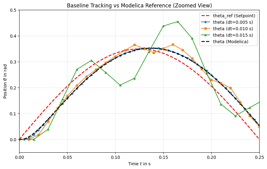
2.12. Plot: Tracking vs Reference#
The plot compares the co-simulation trajectories against the monolithic Modelica reference.
The Modelica reference trajectory is following the reference trajectory closely. The co-simulation trajectories depend strongly on the chosen communication step size, with smaller step sizes generally providing better tracking performance. For dt=0.005s, the co-simulation trajectory closely follows the reference.
t_setpoint = histories['0.005s']['Setpoint'][0]
theta_ref = histories['0.005s']['Setpoint'][1]['theta_ref']

t_005 = histories['0.005s']['Pendulum'][0]
t_010 = histories['0.010s']['Pendulum'][0]
t_015 = histories['0.015s']['Pendulum'][0]

theta_005 = histories['0.005s']['Pendulum'][1]['theta']
theta_010 = histories['0.010s']['Pendulum'][1]['theta']
theta_015 = histories['0.015s']['Pendulum'][1]['theta']
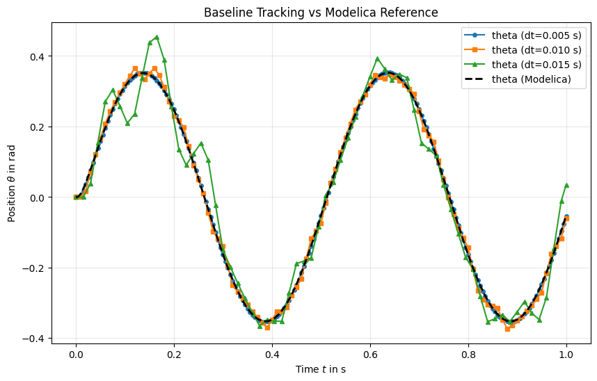
It can be seen that in the start, the co-simulation trajectories with larger step sizes (e.g., dt=0.015s) start oscillating around the reference trajectory. Due to the large communication step size, the controller is not able to react to the changes in the system state quickly enough, leading to overshooting and oscillations. In contrast, the co-simulation trajectory with dt=0.005s closely follows the reference trajectory, indicating that the controller can react more effectively to changes in the system state.
2.13. Summary#
Co-simulation trajectories match the monolithic reference at the baseline settings for sufficient small communication step sizes.
This notebook defines the default parameter set used in later case studies.