

1. Modelica Pendulum: Basics#
This tutorial introduces the pendulum model in Modelica, we simulate it as ModelicaSystem using OMPython and exports it as an FMU for co-simulation with syssimx.
1.1. Overview#
We use one pendulum model in two ways:
Simulate directly with
OMPython.ModelicaSystem.Export to FMI 2.0 Co-Simulation FMUs and simulate with
syssimx.FMUComponent.
In both cases we compare solver behavior under the same constant torque input for different time step sizes.
1.2. Learning Goals#
Understand the pendulum dynamics represented in Modelica.
Understand Modelica block interfaces (
RealInput,RealOutput) for tool integration.Compare solver behavior in direct Modelica simulation (
dassl,cvode,euler).Export FMI 2.0 co-simulation FMUs and compare
cvodevseulerFMU behavior.Understand solver constraints relevant for later hybrid/rollback tutorials.
1.3. Prerequisites and Setup#
import numpy as np
import matplotlib.pyplot as plt

from OMPython import ModelicaSystem
from syssimx import FMUComponent
We are using OpenModelica:
from OMPython import OMCSessionZMQ
omc = OMCSessionZMQ()
omc.sendExpression("getVersion()")
'OpenModelica v1.26.3 (64-bit)'
We are using OMPython version 4.0.0:
!python -m pip show OMPython
Name: OMPython
Version: 4.0.0
Summary: OpenModelica-Python API Interface
Home-page: http://openmodelica.org/
Author:
Author-email: Anand Kalaiarasi Ganeson <ganan642@student.liu.se>
License: This project is part of OpenModelica.

 Copyright (c) 1998-CurrentYear, Open Source Modelica Consortium (OSMC),
 c/o Linköpings universitet, Department of Computer and Information Science,
 SE-58183 Linköping, Sweden.

 All rights reserved.

 THIS PROGRAM IS PROVIDED UNDER THE TERMS OF THE BSD NEW LICENSE OR THE
 GPL VERSION 3 LICENSE OR THE OSMC PUBLIC LICENSE (OSMC-PL) VERSION 1.2.
 ANY USE, REPRODUCTION OR DISTRIBUTION OF THIS PROGRAM CONSTITUTES
 RECIPIENT'S ACCEPTANCE OF THE OSMC PUBLIC LICENSE OR THE GPL VERSION 3,
 ACCORDING TO RECIPIENTS CHOICE.

 The OpenModelica software and the OSMC (Open Source Modelica Consortium)
 Public License (OSMC-PL) are obtained from OSMC, either from the above
 address, from the URLs: http://www.openmodelica.org or
 http://www.ida.liu.se/projects/OpenModelica, and in the OpenModelica
 distribution. GNU version 3 is obtained from:
 http://www.gnu.org/copyleft/gpl.html. The New BSD License is obtained from:
 http://www.opensource.org/licenses/BSD-3-Clause.

 This program is distributed WITHOUT ANY WARRANTY; without even the implied
 warranty of MERCHANTABILITY or FITNESS FOR A PARTICULAR PURPOSE, EXCEPT AS
 EXPRESSLY SET FORTH IN THE BY RECIPIENT SELECTED SUBSIDIARY LICENSE
 CONDITIONS OF OSMC-PL.

Location: c:\Users\flori\anaconda3\envs\env-312\Lib\site-packages
Requires: numpy, psutil, pyparsing, pyzmq
Required-by:
1.4. Physical Model and Governing Equation#
For a pendulum with inertia I, mass m, center-of-mass distance L, gravity g, and applied torque tau, we use
The first-order state form is
Modelica uses a physical/acausal equation-based style: you declare variables and equations, and the tool derives the executable simulation form.
1.5. Modelica Implementation#
The model file defines parameters, one torque input, and three outputs (theta, omega, alpha).
These interface variables are used within the FMUComponent for the definition of the input and output ports.
model Pendulum
  // Imports
  import Modelica.Constants.pi;

  // Parameters
  parameter Real m(unit="kg") = 40;
  parameter Real L(unit="m") = 0.6;
  parameter Real theta0(unit="rad") = 0;
  parameter Real omega0(unit="rad/s") = 0;
  parameter Real g(unit="m/s2") = 9.81;
  parameter Real inertia(unit="kg.m2") = 20;

  // Input torque at the pivot
  Modelica.Blocks.Interfaces.RealInput torque(unit="N.m");

  // Outputs
  Modelica.Blocks.Interfaces.RealOutput theta(unit="rad");
  Modelica.Blocks.Interfaces.RealOutput omega(unit="rad/s");
  Modelica.Blocks.Interfaces.RealOutput alpha(unit="rad/s2") = der(omega);

initial equation
  theta = theta0;
  omega = omega0;

equation
  der(theta) = omega;
  der(omega) = -(m * g * L / inertia) * sin(theta) + torque / inertia;
end Pendulum;
model_file = _repo / "docs/04_tool_integration/01_modelica/models/Pendulum.mo"
1.6. Simulate ModelicaSystem#
# 1. Build the model
modelica_pendulum = ModelicaSystem(
    fileName=str(model_file),
    modelName="Pendulum",
)
modelica_pendulum.buildModel()

# 2. Set parameters
theta0 = 0.0
omega0 = 0.0
modelica_pendulum.setParameters({"theta0": str(theta0), "omega0": str(omega0)})

# 3. Set inputs
torque = 30
modelica_pendulum.setInputs({"torque": f"{torque}"})

# 4. Now simulate — the override file will contain stopTime, stepSize, tolerance
t_stop, dt_ref, tol_ref = 3, 1e-4, 1e-8
modelica_pendulum.simulate(simargs={
    'stopTime':  f"{t_stop}",
    'stepSize':  f"{dt_ref}",
    'tolerance': f"{tol_ref}",
})

# 5. Get results
ref_results = {}
solutions = ('time', 'theta')
for solution in solutions:
     ref_results[solution] = modelica_pendulum.getSolutions(solution).flatten()
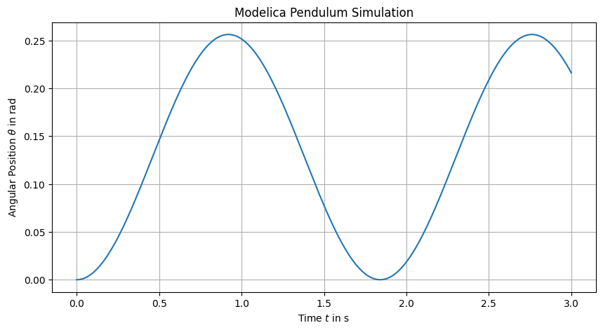
plt.figure(figsize=(10, 5))
plt.plot(ref_results['time'], ref_results['theta'])
plt.xlabel(r'Time $t$ in s')
plt.ylabel(r'Angular Position $\theta$ in rad')
plt.title('Modelica Pendulum Simulation')
plt.grid()
plt.show()
1.7. Export to FMU#
For this workflow we export the ModelicaSystem as FMI 2.0 Co-Simulation FMUs.
By default, the co-simulation FMU exported from OMPython uses euler as the solver. We also create a cvode FMU for comparison.
We specify the solver using the commandLineOptions argument of convertMo2Fmu:
modelica_cvode = ModelicaSystem(
    fileName=str(model_file),
    modelName="Pendulum",
    commandLineOptions=["--fmiFlags=s:cvode"],
)
modelica_cvode.buildModel()

modelica_euler = ModelicaSystem(
    fileName=str(model_file),
    modelName="Pendulum",
    commandLineOptions=["--fmiFlags=s:euler"],
)
modelica_euler.buildModel()

fmu_path_cvode = modelica_cvode.convertMo2Fmu(version="2.0", fmuType="cs")
fmu_path_euler = modelica_euler.convertMo2Fmu(version="2.0", fmuType="cs")
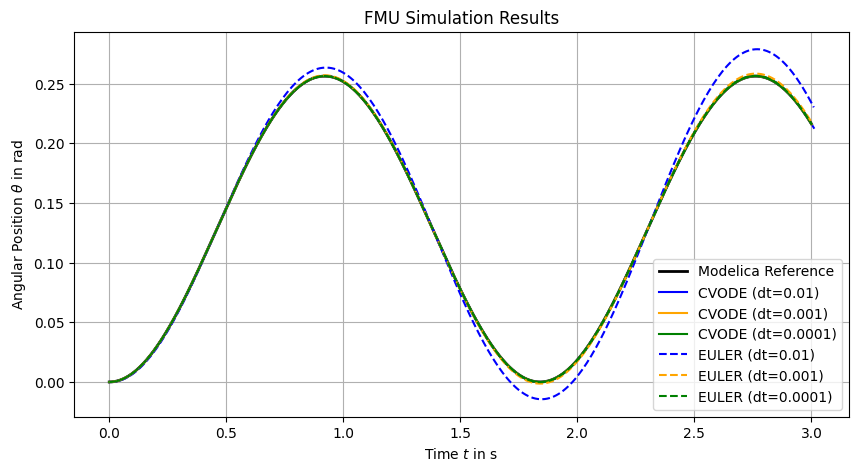
1.8. Simulate FMUComponents#
We run both FMUs with the same initial conditions and same constant torque input. To show step-size effects clearly, we test two communication step sizes.
fmu_components = {
    "cvode": FMUComponent(name="PendulumCVODE", fmu_path=fmu_path_cvode),
    "euler": FMUComponent(name="PendulumEuler", fmu_path=fmu_path_euler),
}

dt_values = [1e-2, 1e-3, 1e-4]

fmu_results = {}

for solver_name, comp in fmu_components.items():
    fmu_results[solver_name] = {}
    for dt in dt_values:
        dt_results = {}
        comp.reset()
        comp.set_parameters(theta0=theta0, omega0=omega0)
        comp.initialize(t0=0.0)
        comp.set_inputs({'torque': torque})
        t_vals = np.arange(0.0, t_stop + dt, dt)
        for t in t_vals:
            comp.do_step(t, dt)
        history = comp.get_history()
        dt_results['theta'] = history['theta']
        fmu_results[solver_name][f"{dt}"] = dt_results
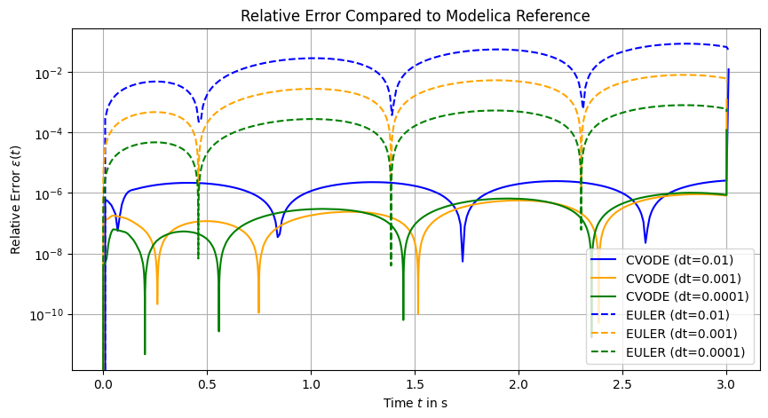
We calculate the relative error compared to the Modelica reference solution for theta:
1.9. Conclusion#
We have simulated the Modelica pendulum model both directly and via FMU co-simulation, comparing solver behaviors and step-size effects.
The figure above shows the relative errors in the pendulum angle theta for different solvers and step sizes compared to the reference solution obtained from the direct Modelica simulation using the dassl solver with a small tolerance.
It can be concluded that:
The
cvodesolver performs significantly better than theeulersolver for the same step sizes.Decreasing the step size improves accuracy for both solvers, but
cvodeachieves lower errors even at larger step sizes.The direct Modelica simulation with
dasslprovides a reliable reference solution for comparison.
We will see in the later tutorials how these solver characteristics impact hybrid simulations and rollback scenarios.