

2. Algebraic Loop System#
This tutorial demonstrates how SysSimX detects and solves algebraic loops.
We build a small feedback system with a direct-feedthrough loop and compare the simulation to an analytic reference.

2.1. Overview#
An algebraic loop occurs when outputs depend instantaneously on inputs in a cycle.
SysSimX detects such loops using dependency graphs and solves them iteratively during each time step.
2.2. Learning Goals#
Identify an algebraic loop created by direct feedthrough
Understand how SysSimX computes execution order and resolves loops
Simulate a system with an algebraic loop and compare to a reference solution
2.2.1. Interface Jacobian-based Algorithm#
The syssimx library implements a modification of the Interface Jacobian-based Co-Simulation Algorithm according to Sicklinger et al. (2014) for solving algebraic loops.
The key steps of the algorithm are shown in the figure below:

References:
S. Sicklinger, V. Belsky, B. Engelmann, H. Elmqvist, H. Olsson, R. Wüchner, and K.-U. Bletzinger.
Interface Jacobian-based Co-Simulation.
International Journal for Numerical Methods in Engineering, 98(4):418–444, 2014.
doi:10.1002/nme.4637.
2.3. Prerequisites and Setup#
We require the following packages:
syssimxnumpymatplotlibgraphviz(for visualization)
import numpy as np
import matplotlib.pyplot as plt

from syssimx import CoSimComponent, Connection, System
from syssimx.core import PortSpec, PortType
from syssimx.viz.system_graph_visualizer import SystemGraphVisualizer
2.4. Implementation#
We define a constant source, two subtractors, and an integrator.
The inner subtractor has direct feedthrough and a self-loop on its input, which creates an algebraic loop.
2.4.1. ConstantSource Component#
Outputs a fixed value.
class ConstantSource(CoSimComponent):
    """A source component that outputs a constant value."""

    def __init__(self, name: str, value: float = 1.0):
        super().__init__(name, group="Source")
        self.value = value
        self.output_specs.update({"y": PortSpec(name="y", type=PortType.REAL, direction="out")})

    def _initialize_component(self, t0: float) -> None:
        pass

    def _do_step_internal(self, t: float, dt: float) -> None:
        pass

    def _update_output_states(self, t: float | None = None, event_names: list[str] | None = None):
        self.outputs["y"].set(self.value, t)
2.4.2. Subtractor Component#
Computes pos - neg.
Because the output depends directly on its inputs, this component has direct feedthrough and participates in algebraic loops.
class Subtractor(CoSimComponent):
    """A subtractor component that subtracts its two input signals.

    diff = input1 - input2
    """
    def __init__(self, name="Subtractor"):
        super().__init__(name, group="Subtractor")
        self.input_specs.update({
            "pos": PortSpec("pos", PortType.REAL, direction="in"),
            "neg": PortSpec("neg", PortType.REAL, direction="in"),
        })
        self.output_specs.update({"diff": PortSpec("diff", PortType.REAL, direction="out")})

    def _initialize_component(self, t0: float) -> None:
        pass

    def _do_step_internal(self, t: float, dt: float) -> None:
        pass

    def _update_output_states(self, t: float | None = None, event_names: list[str] | None = None):
        """Update the output port states based on the current input values."""
        input1_value = self.inputs["pos"].get()
        input2_value = self.inputs["neg"].get()
        self.result = input1_value - input2_value
        self.outputs["diff"].set(self.result, t)

    def evaluate_outputs(self, inputs) -> dict:
        """Evaluate outputs based on given inputs."""
        i1 = inputs.get("pos", self.inputs["pos"].get())
        i2 = inputs.get("neg", self.inputs["neg"].get())
        self.outputs["diff"].set(i1 - i2, None)
        return {"diff": i1 - i2}

    def reset(self):
        super().reset()
        self.outputs["diff"].set(0.0)
2.4.3. Integrator Component#
Accumulates its input over time using explicit Euler stepping.
class Integrator(CoSimComponent):
    """ An integrator component that integrates its input signal u over time.

    The output y(t) is the integral of the input u(t) with respect to time
    """

    def __init__(self, name="Integrator", x0=0.0):
        super().__init__(name, group="Integrator")
        self.input_specs.update({"u": PortSpec(name="u", type=PortType.REAL, direction="in")})
        self.output_specs.update({"y": PortSpec(name="y", type=PortType.REAL, direction="out", unit=None, description="Integrated output")})
        self.x0 = x0

    def _initialize_component(self, t0: float) -> None:
        """Initialize the integrator state."""
        self.x = self.x0

    def _do_step_internal(self, t: float, dt: float) -> None:
        """Perform a simulation step by integrating the input signal."""
        u = self.inputs["u"].get()
        self.x += u * dt

    def _update_output_states(self, t: float | None = None, event_names: list[str] | None = None):
        """Update the output port states."""
        self.outputs["y"].set(self.x, t)

    def reset(self):
        """Reset the integrator state to the initial value."""
        super().reset()
        self.x = self.x0
        self._update_output_states(self.t)
2.5. Instantiation of Components#
We create two subtractors: an outer subtractor for feedback and an inner subtractor that participates in the algebraic loop.
constant_source = ConstantSource(name="ConstSource", value=1.0)

subtractor_inner = Subtractor(name="InnerSubtractor")
subtractor_inner.group = "Algebraic Loop"

subtractor_outer = Subtractor(name="OuterSubtractor")
subtractor_outer.group = "Feedback"

integrator = Integrator(name="Integrator", x0=0.0)

components = [constant_source, subtractor_inner, subtractor_outer, integrator]
2.6. Defining Connections#
The inner subtractor feeds its own negative input, which makes its output implicitly defined:
diff_inner = pos_inner - diff_innerTherefore
diff_inner = 0.5 * pos_inner
This direct-feedthrough self-loop creates an algebraic loop that SysSimX must solve.
# Define connections
c1 = Connection(
    src_comp=constant_source.name,
    src_port=constant_source.output_specs["y"].name,
    dst_comp=subtractor_outer.name,
    dst_port=subtractor_outer.input_specs["pos"].name,
)

c2 = Connection(
    src_comp=subtractor_outer.name,
    src_port=subtractor_outer.output_specs["diff"].name,
    dst_comp=subtractor_inner.name,
    dst_port=subtractor_inner.input_specs["pos"].name,
)
# Algebraic loop connections
c3 = Connection(
    src_comp=subtractor_inner.name,
    src_port=subtractor_inner.output_specs["diff"].name,
    dst_comp=integrator.name,
    dst_port=integrator.input_specs["u"].name,
)

c4 = Connection(
    src_comp=subtractor_inner.name,
    src_port=subtractor_inner.output_specs["diff"].name,
    dst_comp=subtractor_inner.name,
    dst_port=subtractor_inner.input_specs["neg"].name,
)

# Feedback from integrator output to subtractor_outer
c5 = Connection(
    src_comp=integrator.name,
    src_port=integrator.output_specs["y"].name,
    dst_comp=subtractor_outer.name,
    dst_port=subtractor_outer.input_specs["neg"].name,
)

connections = [c1, c2, c3, c4, c5]
2.7. Creating the System#
We add components and connections, then initialize the system. Initialization includes loop detection and solving for a consistent initial state.
2.7.1. Enabling Logging#
SysSimX uses Python’s standard logging module with a NullHandler at the package root — no output is produced unless you explicitly configure a handler in your application.
The following loggers are available:
Logger name |
Content |
|---|---|
|
Algebraic-loop solver iterations and convergence |
|
Hybrid simulation algorithm events |
|
History save / load messages |
|
Multi-model component mode switching |
Setting the syssimx logger to DEBUG activates all of them at once.
For fine-grained control, configure individual sub-loggers instead.
Tip: Use
%(module)sin the format string to display only the filename (e.g.[ijcsa]) instead of the full dotted path. The hierarchical logger names are preserved for filtering — only the display is shortened.
import logging

logging.basicConfig(
    level=logging.WARNING,  # keep third-party loggers quiet
    format="[%(module)s] %(levelname)s: %(message)s",
)
# Enable debug output for the syssimx package
logging.getLogger("syssimx").setLevel(logging.DEBUG)
# Create system and add components and connections
system = System(name="Algebraic Loop System")

for comp in components:
    system.add_component(comp)

for conn in connections:
    system.add_connection(conn)

system.initialize(t0=0.0)
[ijcsa] DEBUG: Solving algebraic SCC ['InnerSubtractor']:
[ijcsa] DEBUG: Interface inputs: [('InnerSubtractor', 'neg')]
[ijcsa] DEBUG: Internal zero-delay connections [('InnerSubtractor', 'diff', 'InnerSubtractor', 'neg')]
[ijcsa] DEBUG: External zero-delay inputs [('OuterSubtractor', 'diff', 'InnerSubtractor', 'pos')]
[ijcsa] DEBUG: Initial guess for InnerSubtractor.neg = -0.001
[ijcsa] DEBUG: Starting IJCSA iterations:
[ijcsa] DEBUG:   Iteration 0: u = [-0.001]
[ijcsa] DEBUG:     Residual for InnerSubtractor.neg: -1.0019999999999998
[ijcsa] DEBUG:     Residual for InnerSubtractor.neg: -1.001998
[ijcsa] DEBUG:     Jacobian J = [[2.]]
[ijcsa] DEBUG:     Correction Δu = [0.501]
[ijcsa] DEBUG:   Iteration 1: u = [0.5]
[ijcsa] DEBUG:     Residual for InnerSubtractor.neg: 8.243095095394892e-11
[ijcsa] DEBUG:   Converged in 1 iterations.
[ijcsa] DEBUG: Committed solved input InnerSubtractor.neg = 0.5000000000412155
The debug output above shows the IJCSA solver at work:
It identifies the algebraic SCC containing
InnerSubtractorIt lists the interface inputs and internal zero-delay connections
It iterates (Newton step) until the residual is below tolerance
It commits the converged input values
To silence the output again, raise the log level:
# Silence syssimx logging for the rest of the notebook
logging.getLogger("syssimx").setLevel(logging.WARNING)
2.8. Inspecting the Structure#
The structural report confirms what the solver log showed: the strongly connected component ['InnerSubtractor'] is detected as an algebraic loop, and the direct-feedthrough relations of both subtractors are listed.
print(system.describe())
System 'Algebraic Loop System'
  Algorithm: GaussSeidelAlgorithm
  Initialized: True
  Components (4):
    - ConstSource (ConstantSource): 0 in / 1 out
    - InnerSubtractor (Subtractor): 2 in / 1 out [direct feedthrough]
    - OuterSubtractor (Subtractor): 2 in / 1 out [direct feedthrough]
    - Integrator (Integrator): 1 in / 1 out
  Connections (5):
    - ConstSource.y -> OuterSubtractor.pos
    - OuterSubtractor.diff -> InnerSubtractor.pos
    - InnerSubtractor.diff -> Integrator.u
    - InnerSubtractor.diff -> InnerSubtractor.neg
    - Integrator.y -> OuterSubtractor.neg
  Execution order:
    Generation 0: ConstSource, Integrator
    Generation 1: OuterSubtractor
    Generation 2: InnerSubtractor
  Algebraic loops (1):
    - InnerSubtractor
2.9. Visualizing the System Graph#
The system graph highlights the algebraic loop. Direct-feedthrough outputs are shown in red.
visualizer = SystemGraphVisualizer(system)
visualizer.visualize("figures/algebraic_loop_graph.svg")

2.10. Initial Consistent State#
After initialization, SysSimX has solved the algebraic loop to produce consistent outputs.
print(60 * "=", "\nInitial consistent system state:")
print("Source;           ", constant_source.get_outputs())
print("Outer Subtractor: ", subtractor_outer.get_outputs())
print("Inner Subtractor: ", subtractor_inner.get_outputs())
print("Integrator:       ", integrator.get_outputs())
============================================================
Initial consistent system state:
Source;            {'y': 1.0}
Outer Subtractor:  {'diff': 1.0}
Inner Subtractor:  {'diff': 0.4999999999587845}
Integrator:        {'y': 0.0}
2.11. Running the Simulation#
We simulate for 10 seconds with a fixed time step.
t0 = 0.0
tf = 10.0
dt = 0.01

result = system.run(t0=t0, tf=tf, dt=dt)
result
<SimulationResult 'Algebraic Loop System' t=[0.0, 10.0] dt=0.01 components=4 algorithm=GaussSeidelAlgorithm>
2.12. Retrieving the Results#
system.run() returns a SimulationResult; we take the integrator and inner-subtractor histories from it for plotting.
t_integrator, data_integrator = result["Integrator"]
y_integrator = data_integrator["y"]
t_inner_subtractor, data_inner_subtractor = result["InnerSubtractor"]
diff_inner_subtractor = data_inner_subtractor["diff"]
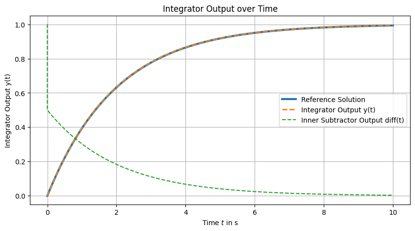
2.13. Reference Solution#
The system reduces to the ODE:
with analytic solution:
dt_ref = dt / 100
t_ref = np.arange(t0, tf + dt_ref, dt_ref)
y_ref = 1 - np.exp(-0.5 * t_ref)
2.14. Visualizing the Results#
The figure below shows the integrator output converging to the reference solution, demonstrating that SysSimX successfully solved the algebraic loop at each time step.
2.15. Conclusion#
This example shows how SysSimX detects and resolves algebraic loops automatically, allowing stable simulation of coupled direct-feedthrough components. The loop is visible in three places: the IJCSA solver log during initialization, the describe() report, and the red direct-feedthrough ports in the system graph.
2.16. Next Steps#
Simple Hybrid System — discrete events and the hybrid master algorithm.
Algebraic Loop — an algebraic loop in the full controlled-pendulum benchmark, including a PID parameter study.