

2. Quickstart#
This quickstart builds a tiny system with a linear source feeding an integrator. You will connect the components, run a simulation, and plot the results.
2.1. Import SysSimX#
We use the CoSimComponent, System, and Connection classes, plus matplotlib for plotting.
import numpy as np
import matplotlib.pyplot as plt

from syssimx import CoSimComponent, Connection, System, SystemGraphVisualizer
from syssimx.core import PortSpec, PortType
2.2. Define the Components#
We define a linear source y = a * t + b and a simple integrator that accumulates its input over time.
class LinearSource(CoSimComponent):
    """Linear source: y(t) = a * t + b."""

    def __init__(self, name: str, a: float = 1.0, b: float = 0.0):
        super().__init__(name, group="Source")
        self.a = a
        self.b = b
        self.output_specs.update({
            "y": PortSpec(name="y", type=PortType.REAL, direction="out")
        })

    def _initialize_component(self, t0: float) -> None:
        pass

    def _do_step_internal(self, t: float, dt: float) -> None:
        pass

    def _update_output_states(self, t: float | None = None, event_names=None):
        self.outputs["y"].set(self.a * t + self.b, t)


class Integrator(CoSimComponent):
    """Integrator with explicit Euler stepping."""

    def __init__(self, name: str, x0: float = 0.0):
        super().__init__(name, group="Integrator")
        self.x0 = x0
        self.input_specs.update({
            "u": PortSpec(name="u", type=PortType.REAL, direction="in")
        })
        self.output_specs.update({
            "y": PortSpec(name="y", type=PortType.REAL, direction="out")
        })

    def _initialize_component(self, t0: float) -> None:
        self.x = self.x0

    def _do_step_internal(self, t: float, dt: float) -> None:
        u = self.inputs["u"].get()
        self.x += u * dt

    def _update_output_states(self, t: float | None = None, event_names=None):
        self.outputs["y"].set(self.x, t)
2.3. Build the System#
We connect the source output to the integrator input and initialize the system.
source = LinearSource(name="LinearSource", a=1.0, b=0.0)
integrator = Integrator(name="Integrator", x0=0.0)

system = System(name="QuickstartSystem")
system.add_component(source)
system.add_component(integrator)

system.add_connection(Connection(
    src_comp=source.name,
    src_port=source.output_specs["y"].name,
    dst_comp=integrator.name,
    dst_port=integrator.input_specs["u"].name,
))

system.initialize(t0=0.0)
2.4. Inspect the System#
system.describe() prints a structural report of the assembled system: components, connections, the computed execution order, detected algebraic loops, and the selected master algorithm. Since the system is already initialized, the execution order is included.
print(system.describe())
2.5. Visualize the System Graph#
visualizer = SystemGraphVisualizer(system)
visualizer.visualize()
visualizer.save("first_system_graph.svg")

2.6. Run the Simulation#
We simulate for 5 seconds with a fixed step size. system.run() returns a SimulationResult that bundles the recorded component histories with run metadata (time span, macro step, wall time, algorithm).
t0 = 0.0
tf = 5.0
dt = 0.1

result = system.run(t0=t0, tf=tf, dt=dt)
2.7. Work With the Result#
The returned SimulationResult is the recommended way to access simulation outputs:
result["Integrator"]returns(time_array, {port: values})for one component.result.to_dataframe()returns a tidy long-format pandas DataFrame (component,port,time,value);result.to_dataframe(component="Integrator")returns a wide DataFrame with one column per output port.result.to_csv("run.csv")exports the same data to CSV.result.eventsholds the recorded event log, andresult.wall_time,result.algorithm,result.dtexpose the run metadata.
result
result.to_dataframe(component="Integrator").head()
2.8. Visualize Results#
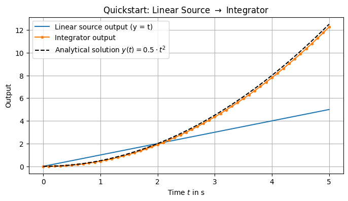
The integrator output is the integral of the linear source. For a=1 and b=0, the expected shape is quadratic.
y_analytical = lambda t: 0.5 * t**2
dt_an = 1e-4
t_vals_an = np.arange(t0, tf + dt_an, dt_an)
y_analytical_vals = y_analytical(t_vals_an)
t_vals, data = result["Integrator"]
y_vals = data["y"]
2.9. Next Steps#
Explore more example systems in the Fundamentals chapter.
See Simple System for a slightly larger system with feedback.
See Importing FMUs for Co-Simulation for loading FMU components.
Systems can also be defined declaratively in YAML/JSON and run from the command line — see Declarative System Descriptions.