

1. Simple Pendulum Component#
1.1. Overview#
In this tutorial we implement a minimal CoSimComponent and run a single-component simulation.
The goal is to learn the interface: define ports, initialize state, advance one time step, and update outputs.
We also add a torque input to show how external inputs are supplied.
1.2. Learning Goals#
Identify the three required hooks:
_initialize_component,_do_step_internal, and_update_output_statesDefine input and output ports and parameters
Run a single-component simulation and inspect time-series outputs
Modify parameters and rerun the simulation
1.3. Prerequisites and Setup#
You have installed
syssimxand its Python dependenciesYou have
numpyandmatplotlibavailableYou are comfortable running Jupyter Notebook cells
This tutorial is self-contained and does not require any FMU files
import numpy as np
import matplotlib.pyplot as plt

from syssimx import CoSimComponent
from syssimx.core.port import PortSpec, PortType
from syssimx.utilities import Quantity
1.4. Model Equations#
We model a simple pendulum with angle theta and angular velocity omega. An external torque tau is applied at the pivot.
where:
\(m\) is the mass of the pendulum
\(g\) is the gravitational acceleration
\(L\) is the length of the pendulum
\(I\) is the moment of inertia about the pivot
\(\tau\) is the external torque input We integrate these equations with explicit Euler time stepping.

Figure: A simple pendulum under the influence of gravity. Source: Wikipedia
#/media/File:Pendulum_gravity.svg)
1.5. Model Definition#
State variables:
theta: angle (rad)omega: angular velocity (rad/s)
Input:
tau: external torque at the pivot (N*m)
Outputs:
theta,omega, andalpha(angular acceleration)
Initial conditions are provided by parameters q0 and omega0.
1.6. Implementation as CoSimComponent#
We define a SimplePendulum component with input and output ports and parameters. The three required hooks are:
_initialize_component: set initial state_do_step_internal: advance the state by one time step_update_output_states: publish outputs
1.6.1. Define the Component Class#
Construction
Define parameters and ports.
Store internal state variables.
Time stepping
Use explicit Euler to advance the state.
Output updates
Write
theta,omega, andalphato the output ports.
Reset
Restore default parameters and clear internal state.
class Pendulum(CoSimComponent):

    def __init__(self, name, label=None, group=None):
        super().__init__(name, label, group)

        self._theta = 0.0
        self._omega = 0.0
        self._alpha = 0.0

        self.input_specs.update({
            "tau": PortSpec(name="tau", type=PortType.REAL, direction="in", unit="N*m"),
        })
        self.output_specs.update({
            "theta": PortSpec(name="theta", type=PortType.REAL, direction="out", unit="rad"),
            "omega": PortSpec(name="omega", type=PortType.REAL, direction="out", unit="rad/s"),
            "alpha": PortSpec(name="alpha", type=PortType.REAL, direction="out", unit="rad/s^2"),
        })

        self._set_default_parameter_values()

    def _set_default_parameter_values(self):
        self.parameters.update({
            "L": Quantity(0.6, "m"),
            "m": Quantity(40, "kg"),
            "inertia": Quantity(20, "kg*m^2"),
            "g": Quantity(9.81, "m/s^2"),
            "q0": Quantity(0.0, "rad"),
            "omega0": Quantity(0.0, "rad/s"),
        })

    def _pendulum_dynamics(self, y: np.ndarray, tau: float):
        theta, omega = y
        m = self.parameters["m"].magnitude
        g = self.parameters["g"].magnitude
        L = self.parameters["L"].magnitude
        I = self.parameters["inertia"].magnitude

        alpha = -(m * g * L * np.sin(theta)) / I + tau / I
        return np.array([omega, alpha])

    def _initialize_component(self, t0):
        self._theta = self.parameters["q0"].magnitude
        self._omega = self.parameters["omega0"].magnitude
        y = np.array([self._theta, self._omega])
        self._alpha = self._pendulum_dynamics(y, tau=0.0)[1]

    def _update_output_states(self, t: float | None = None, event_names: list[str] | None = None):
        self.outputs["theta"].set(self._theta, t)
        self.outputs["omega"].set(self._omega, t)
        self.outputs["alpha"].set(self._alpha, t)

    def _do_step_internal(self, t, dt):
        tau = self.inputs["tau"].get().magnitude
        y = np.array([self._theta, self._omega])
        dydt = self._pendulum_dynamics(y, tau)
        y_next = y + dt * dydt

        self._theta, self._omega = y_next
        self._alpha = self._pendulum_dynamics(y_next, tau)[1]

    def reset(self):
        super().reset()

        self.parameters.clear()
        self._set_default_parameter_values()

        self._theta = 0.0
        self._omega = 0.0
        self._alpha = 0.0
1.6.2. Create an Instance of the Pendulum Component#
pendulum = Pendulum("MyFirstPendulum")
1.6.3. Modifying Model Parameters#
#pendulum.set_parameters(q0=0.3)
original_params = pendulum.get_parameters()
print("Default Parameters:")
for key, value in original_params.items():
    print(f"{key:>10}: {value}")
Default Parameters:
         L: 0.6 m
         m: 40 kg
   inertia: 20 kg·m²
         g: 9.81 m/s²
        q0: 0.0 rad
    omega0: 0.0 rad/s
We can modify the model parameters of the component using the set_parameters method.
Option 1: Set value of a Quantity parameter
Pass the new magnitude directly as a keyword argument.
This assumes the default unit defined in the component.
Option 2: Set value using Quantity
Create a
Quantityobject with the desired magnitude and unit.
Option 3: Set parameter using a compatible unit
Create a
Quantityobject with a different but compatible unit (e.g., centimeters instead of meters).The
set_parametersmethod will handle the unit conversion automatically.
# Option 1: Set value of a Quantity parameter, assuming default unit
pendulum.set_parameters(L=0.8)
print('Option 1:', pendulum.get_parameters('L'))

# Option 2: Set value using Quantity
L = Quantity(0.5, 'm')
pendulum.set_parameters(L=L)
print('Option 2:', pendulum.get_parameters('L'))

# Option 3: Set value using Quantity with different unit
L_cm = Quantity(60, 'cm')  # 60 centimeters
pendulum.set_parameters(L=L_cm)
print('Option 3:', pendulum.get_parameters('L'))

# Retrieving error for unit mismatch
try:
    pendulum.set_parameters(L=Quantity(2, 'kg'))  # Unit mismatch
except Exception as e:
    print(f'Error: {e}')
Option 1: {'L': <Quantity(0.8, 'meter')>}
Option 2: {'L': <Quantity(0.5, 'meter')>}
Option 3: {'L': <Quantity(0.6, 'meter')>}
Error: Parameter 'L' expects units compatible with 'm', got 'kg'.
You can retrieve multiple parameters at once by passing an unpacked list of parameter names to get_parameters(*args) or set several parameters by passing a dictionary to set_parameters.
batch_parameters = pendulum.get_parameters(*['L', 'm', 'g'])
print("Batch Retrieved Parameters:")
for key, value in batch_parameters.items():
    print(f"{key:>10}: {value}")
Batch Retrieved Parameters:
         L: 0.6 m
         m: 40 kg
         g: 9.81 m/s²
new_params = {
    'L': Quantity(1.0, 'm'),
    'm': Quantity(2.0, 'kg'),
    'g': Quantity(9.81, 'm/s^2')
}
pendulum.set_parameters(**new_params)
updated_params = pendulum.get_parameters(*new_params.keys())
print("Batch Updated Parameters:")
for key, value in updated_params.items():
    print(f"{key:>10}: {value}")

pendulum.set_parameters(**original_params)  # Reset to original parameters
print("\nParameters Reset to Original:")
for key, value in pendulum.get_parameters().items():
    print(f"{key:>10}: {value}")
Batch Updated Parameters:
         L: 1.0 m
         m: 2.0 kg
         g: 9.81 m/s²

Parameters Reset to Original:
         L: 0.6 m
         m: 40 kg
   inertia: 20 kg·m²
         g: 9.81 m/s²
        q0: 0.0 rad
    omega0: 0.0 rad/s
1.6.4. Run the Simulation#
We simulate for 5 seconds with a fixed step size of 1 ms. Because this tutorial focuses on the component interface, we drive the component directly with do_step in a loop — no System is involved yet.
t0 = 0.0
time_end = 5
dt = 1e-3
time_points = np.arange(0.0, time_end, dt)
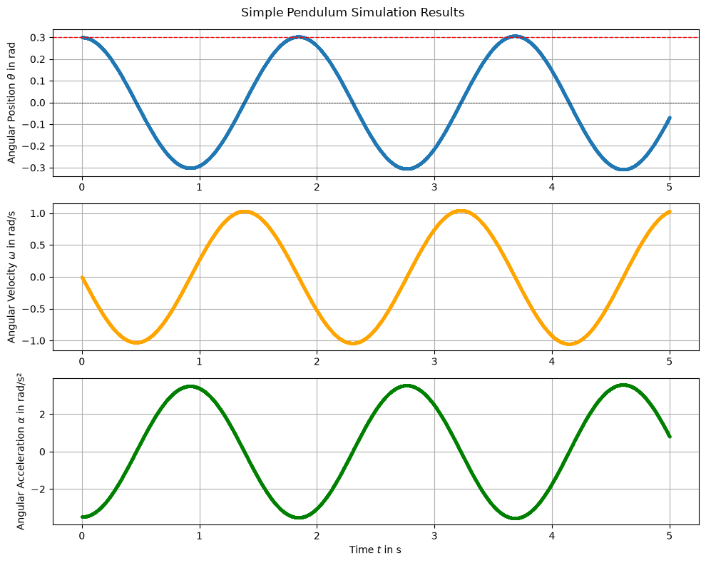
1.6.4.1. Free Swing#
First, we simulate the pendulum without any external torque to observe its free swing.
We define an initial angular position q0 = 0.3 rad and zero initial angular velocity omega0 = 0 rad/s.
pendulum.reset()
pendulum.set_parameters(q0=0.3)
pendulum.initialize(t0)

for t in time_points:
    pendulum.do_step(t, dt)
Retrieve history and plot the results
history = pendulum.get_history()

times = history["theta"]['time']
thetas = history["theta"]['values']
omegas = history["omega"]['values']
alphas = history["alpha"]['values']
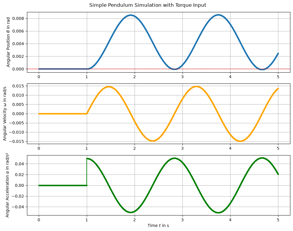
1.6.4.2. With External Torque#
A small torque step is applied after 1 second to demonstrate how inputs are provided to a component.
pendulum.reset()
pendulum.initialize(t0)

def torque_input(t):
    return 1 if t >= 1.0 else 0.0

for t in time_points:
    pendulum.set_inputs({"tau": torque_input(t)}, t=t)
    pendulum.do_step(t, dt)
Retrieve history and plot the results
history = pendulum.get_history()

times = history["theta"]['time']
thetas = history["theta"]['values']
omegas = history["omega"]['values']
alphas = history["alpha"]['values']
1.7. Comparing Parameter Configurations#
pendulum.reset()
default_config = pendulum.get_parameters()
print("Default Parameters:")
for k, v in default_config.items():
    print(f" - {k}: {v}")
Default Parameters:
 - L: 0.6 m
 - m: 40 kg
 - inertia: 20 kg·m²
 - g: 9.81 m/s²
 - q0: 0.0 rad
 - omega0: 0.0 rad/s
pendulum.reset()
default_config = pendulum.get_parameters()

config1 = {
    'L': 2 * default_config['L'],
    'm': 2 * default_config['m'],
}

config2 = {
    'L': 0.5 * default_config['L'],
    'm': 0.5 * default_config['m']
}

labels = ['Default', 'Config 1 -  $2L, 2m$', 'Config 2 - $L/2, m/2$']
configs = [default_config, config1, config2]
histories = []
for i, config in enumerate(configs):
    pendulum.reset()
    pendulum.set_parameters(**config)

    pendulum.initialize(t0=0.0)
    for t in time_points:
        pendulum.set_inputs({'tau': torque_input(t)}, t=t)
        pendulum.do_step(t, dt)

    histories.append(pendulum.get_history())
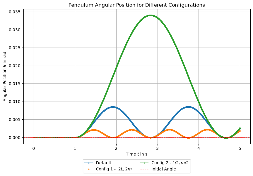
This comparison shows how changes in length and mass affect the pendulum motion.
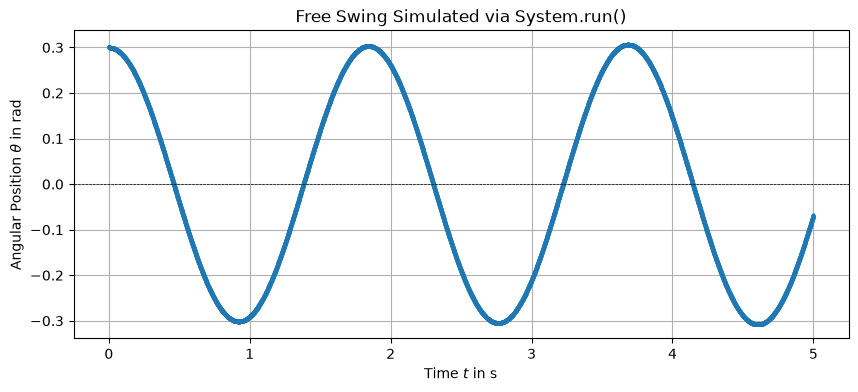
1.8. Running the Component in a System#
Driving do_step by hand is instructive, but in practice components run inside a System, which handles initialization, stepping, and history recording. system.run() returns a SimulationResult with the recorded outputs and run metadata. The unconnected tau input defaults to zero, so this reproduces the free swing.
from syssimx import System

free_pendulum = Pendulum("Pendulum")
free_pendulum.set_parameters(q0=0.3)

system = System(name="PendulumSystem")
system.add_component(free_pendulum)
system.initialize(t0=0.0)

result = system.run(t0=0.0, tf=5.0, dt=1e-3)
result
<SimulationResult 'PendulumSystem' t=[0.0, 5.0] dt=0.001 components=1 algorithm=GaussSeidelAlgorithm>
t_vals, data = result["Pendulum"]

plt.figure(figsize=(10, 4))
plt.plot(t_vals, data["theta"], **style)
plt.axhline(0, color='black', linewidth=0.5, linestyle='--')
plt.title('Free Swing Simulated via System.run()')
plt.xlabel(r'Time $t$ in s')
plt.ylabel(r'Angular Position $\theta$ in rad')
plt.grid()
plt.show()
1.9. Conclusion#
In this tutorial, we implemented a minimal pendulum model as a CoSimComponent and focused on the three required hooks: _initialize_component, _do_step_internal, and _update_output_states.
We defined input and output ports, set parameters with automatic unit handling, ran a manually stepped simulation with an external torque input, and finally ran the same component inside a System, obtaining a SimulationResult.
1.10. Next Steps#
Importing FMUs for Co-Simulation — replace the hand-written component with a Modelica FMU.
Simple System — connect several components into a system with feedback.
Declarative System Descriptions — assemble the same kind of system from a YAML description instead of Python code.