3. Quantization and Sampling#

3.1. Goal#

Show how encoder/decoder resolution and sampling period affect tracking accuracy.

3.2. Model Map#

System Graph

3.3. Assumptions and Scope#

  • No wall contact

  • Fixed-step co-simulation; reference uses variable-step DASSL

3.4. Prerequisites and Setup#

from pathlib import Path
import sys

import numpy as np
import matplotlib.pyplot as plt

from demos.ControlledPendulum.src.master_pendulum import MasterPendulum
import demos.ControlledPendulum.src.master_pendulum.components.fem.pendulum_config as config

from syssimx import FMUComponent, Connection, System, SystemGraphVisualizer

3.5. Discover FMUs#

PLATFORM = sys.platform
demo_dir_path = Path().cwd() / "demos" / "ControlledPendulum"
package_path = Path(demo_dir_path / "src/modelica/ControlledPendulum")
fmu_output_dir = Path(demo_dir_path / f"artifacts/fmus/{PLATFORM}")

fmu_paths = {}
for subdir in fmu_output_dir.iterdir():
    if subdir.is_dir():
        fmu_paths[subdir.name] = {}
        for fmu_file in subdir.glob("*.fmu"):
            fmu_paths[subdir.name][fmu_file.stem] = fmu_file
        for subsubdir in subdir.iterdir():
            fmu_paths[subdir.name][subsubdir.name] = {}
            if subsubdir.is_dir():
                fmu_paths[subdir.name][subsubdir.name] = {}
                for fmu_file in subsubdir.glob("*.fmu"):
                    fmu_paths[subdir.name][subsubdir.name][fmu_file.stem] = fmu_file
    else:
        fmu_paths[subdir.stem] = subdir

3.6. Modelica Reference Simulation#

We refer to the monolithic Modelica simulation as “Modelica” in the following. The simulation results are obtained by running the Quantization example model in OpenModelica using the OMPython interface. The model can be found in the ControlledPendulum package

from OMPython import ModelicaSystem

reference = ModelicaSystem(fileName=str(package_path / "package.mo"),
                           modelName="ControlledPendulum.Examples.NoContact.Quantization")
reference.buildModel()

Hide code cell output

Notification: Automatically loaded package Complex 4.0.0 due to uses annotation from Modelica.
Notification: Automatically loaded package ModelicaServices 4.0.0 due to uses annotation from Modelica.
Notification: Automatically loaded package Modelica 4.0.0 due to usage.

3.6.1. Reference Sensor Parameters#

ref_params = reference.getParameters()

ref_sensor_params = {
    "nBits": int(ref_params['angle_sensor.nBits']),
    "samplePeriod": float(ref_params['angle_sensor.samplePeriod']),
    "decoder_nBits": int(ref_params['angle_decoder.nBits']),
    "decoder_samplePeriod": float(ref_params['angle_decoder.samplePeriod']),
}

print("Reference sensor parameters →")
print(f"  nBits: {ref_sensor_params['nBits']}")
print(f"  samplePeriod [s]: {ref_sensor_params['samplePeriod']}")
Reference sensor parameters →
  nBits: 10
  samplePeriod [s]: 0.01

3.6.2. Run Reference Simulation#

reference.simulate()
ref_sol_names = ('time', 'theta', 'theta_meas')
ref_sol = {name: reference.getSolutions(name).flatten() for name in ref_sol_names}
LOG_SUCCESS       | info    | The initialization finished successfully without homotopy method.
LOG_SUCCESS       | info    | The simulation finished successfully.

3.7. Instantiate FMU Components#

def print_parameteres(component: FMUComponent):
    print(f"Parameters of {component.name}:")
    for name, param in component.parameters.items():
        if '.' not in name and param is not None:
            print(f"  - {name}: {param}")

3.7.1. Setpoint#

setpoint = FMUComponent(name="Setpoint",
                         fmu_path=fmu_paths['Trajectories']["SetPoint"],
                         group="Reference")
print_parameteres(setpoint)
Parameters of Setpoint:
  - amplitude: 0.3490658503988659 rad
  - frequency: 0.75 Hz
  - offset: 0.0 rad
  - phase: 0.0 rad

3.7.2. PID Controller#

pid = FMUComponent(name="PID",
                   fmu_path=fmu_paths['Controllers']["PIDController"],
                   group="Controller")
print_parameteres(pid)
Parameters of PID:
  - Kd: 0.15
  - Ki: 4.0
  - Kp: 10.0
  - uMax: 1.0
  - uMin: -1.0

3.7.3. Drive#

drive = FMUComponent(name="Drive",
                     fmu_path=fmu_paths['Actuators']["DriveDynamic"],
                     group="Actuator")
print_parameteres(drive)
Parameters of Drive:
  - I_max: 10.0 A
  - L_arm: 0.000121 H
  - R_arm: 0.151 Ohm
  - V_rated: 48.0 V
  - V_supply: 16.0 V
  - eta: 0.85
  - gearRatio: 60.0
  - k_t: 0.03 m·N/A
  - n_0: 12916.0 1/min

3.7.4. Pendulum#

pendulum = FMUComponent(name="Pendulum",
                        fmu_path=fmu_paths['Plants']["Pendulum_cvode"],
                        group="Plant")
print_parameteres(pendulum)
Parameters of Pendulum:
  - J: 0.442268222 kg·m²
  - L: 0.181650853 m
  - b_viscous: 0.0 m·N·s/rad
  - g: 9.81 m/s²
  - m: 10.8429606 kg
  - omega_eps: 0.001 rad/s
  - omega_start: 0.0 rad/s
  - tau_c: 0.0 m·N
  - theta_start: 0.0 rad

3.7.5. Angle Sensor and Decoder#

angle_sensor = FMUComponent(name="Angle Sensor",
                             fmu_path=fmu_paths['Sensors']['AngleSensor'],
                             group="Sensors")
print_parameteres(angle_sensor)
Parameters of Angle Sensor:
  - pot_range: 4.71238898038469 rad
  - r_bottom: 20000.0 Ohm
  - r_top: 80000.0 Ohm
  - samplePeriod: 0.01 s
  - theta_max: 0.45378560551852565 rad
  - theta_min: -0.45378560551852565 rad
  - v_adc: 3.0 V
  - v_pot: 5.0 V
  - nBits: 10
angle_decoder = FMUComponent(name="Angle Decoder",
                             fmu_path=fmu_paths['Sensors']['AngleDecoder'],
                             group="Signal Processing")

print_parameteres(angle_decoder)
Parameters of Angle Decoder:
  - pot_range: 4.71238898038469 rad
  - r_bottom: 20000.0 Ohm
  - r_top: 80000.0 Ohm
  - samplePeriod: 0.01 s
  - theta_max: 0.45378560551852565 rad
  - theta_min: -0.45378560551852565 rad
  - v_adc: 3.0 V
  - v_pot: 5.0 V
  - nBits: 10

3.8. Define Connections#

c1 = Connection(
    src_comp=setpoint.name,
    src_port=setpoint.output_specs["theta_ref"].name,
    dst_comp=pid.name,
    dst_port=pid.input_specs["theta_ref"].name,
)

c2 = Connection(
    src_comp=pendulum.name,
    src_port=pendulum.output_specs["theta"].name,
    dst_comp=angle_sensor.name,
    dst_port=angle_sensor.input_specs["theta"].name,
)

c3 = Connection(
    src_comp=angle_sensor.name,
    src_port=angle_sensor.output_specs["v_out"].name,
    dst_comp=angle_decoder.name,
    dst_port=angle_decoder.input_specs["v_in"].name,
)

c4 = Connection(
    src_comp=angle_decoder.name,
    src_port=angle_decoder.output_specs["theta"].name,
    dst_comp=pid.name,
    dst_port=pid.input_specs["theta_meas"].name,
)

c5 = Connection(
    src_comp=pid.name,
    src_port=pid.output_specs["u"].name,
    dst_comp=drive.name,
    dst_port=drive.input_specs["u_control"].name,
)

c6 = Connection(
    src_comp=drive.name,
    src_port=drive.output_specs["torque"].name,
    dst_comp=pendulum.name,
    dst_port=pendulum.input_specs["tau"].name,
)

c7 = Connection(
    src_comp=pendulum.name,
    src_port=pendulum.output_specs["omega"].name,
    dst_comp=drive.name,
    dst_port=drive.input_specs["omega"].name,
)

connections = [c1, c2, c3, c4, c5, c6, c7]
components = [setpoint, pid, drive, angle_sensor, angle_decoder, pendulum]

3.9. Build and Initialize the System#

system = System(name="Pendulum System with Quantization")

for comp in components:
    system.add_component(comp)

for conn in connections:
    system.add_connection(conn)

system.initialize(t0=0.0)

Hide code cell output

LOG_SOLVER        | info    | CVODE linear multistep method CV_BDF
LOG_SOLVER        | info    | CVODE maximum integration order CV_ITER_NEWTON
LOG_SOLVER        | info    | CVODE use equidistant time grid YES
LOG_SOLVER        | info    | CVODE Using relative error tolerance 1.000000e-06
LOG_SOLVER        | info    | CVODE Using dense internal linear solver SUNLinSol_Dense.
LOG_SOLVER        | info    | CVODE Use internal dense numeric jacobian method.
LOG_SOLVER        | info    | CVODE uses internal root finding method NO
LOG_SOLVER        | info    | CVODE maximum absolut step size 0
LOG_SOLVER        | info    | CVODE initial step size is set automatically
LOG_SOLVER        | info    | CVODE maximum integration order 5
LOG_SOLVER        | info    | CVODE maximum number of nonlinear convergence failures permitted during one step 10
LOG_SOLVER        | info    | CVODE BDF stability limit detection algorithm OFF

3.10. Visualize the System Graph#

visualizer = SystemGraphVisualizer(system)
visualizer.visualize()
../_images/3c3a39eb1d04ca2d68b76004da168c08a9e29256954f72a3cf43ea0bddf505ee.svg

3.11. Baseline Run#

angle_sensor.set_parameters(
    nBits=ref_sensor_params["nBits"],
    samplePeriod=ref_sensor_params["samplePeriod"],
)
angle_decoder.set_parameters(
    nBits=ref_sensor_params["decoder_nBits"],
    samplePeriod=ref_sensor_params["decoder_samplePeriod"],
)

t = 0.0
dt = 0.001
t_end = 2

system.run(t, t_end, dt)

print(f"Simulation config → dt [s]: {dt}, t_end [s]: {t_end}, nBits: {ref_sensor_params['nBits']}, samplePeriod [s]: {ref_sensor_params['samplePeriod']}")
Simulation config → dt [s]: 0.001, t_end [s]: 2, nBits: 10, samplePeriod [s]: 0.01

3.12. Collect Results#

history = system.get_history()

t_setpoint = history["Setpoint"][0]
theta_ref = history["Setpoint"][1]["theta_ref"]

t_pendulum = history["Pendulum"][0]
theta_pendulum = history["Pendulum"][1]["theta"]

t_decoder = history["Angle Decoder"][0]
theta_decoder = history["Angle Decoder"][1]["theta"]

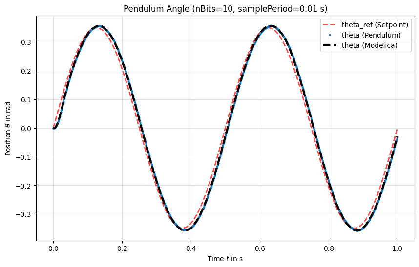
3.13. Plot: Baseline Tracking vs Reference#

This baseline uses the reference sensor settings.

plt.figure(figsize=(10, 6))
plt.plot(t_setpoint, theta_ref, label="theta_ref (Setpoint)", color='red', linestyle='--', linewidth=2)
plt.plot(t_pendulum, theta_pendulum, 'o', label="theta (Pendulum)", markersize=2)
plt.plot(ref_sol['time'], ref_sol['theta'], label="theta (Modelica)", color='black', linestyle=':', linewidth=2)
plt.xlabel(r"Time $t$  [s]")
plt.ylabel(r"Angular Position $\theta$  [rad]")
plt.title(f"Pendulum Angle (nBits={ref_sensor_params['nBits']}, samplePeriod={ref_sensor_params['samplePeriod']} s)")
plt.legend()
plt.grid(True, alpha=0.3)
plt.show()
../_images/f04d26eef5590f62e4c4e19d61dbe6bffc6928f3882254bbbb382837d8cfcfca.png
plt.figure(figsize=(10, 6))
plt.plot(t_setpoint, theta_ref, label="theta_ref", color='red', linestyle='--', linewidth=2)
plt.plot(t_decoder, theta_decoder, 'o', label="theta_meas", markersize=2)
plt.plot(ref_sol['time'], ref_sol['theta_meas'], 'o', label="theta_meas (Modelica)", color='black', markersize=2)
plt.xlim(0, 0.5)
plt.ylim(-0.05, 0.4)
plt.xlabel(r"Time $t$  [s]")
plt.ylabel(r"Angular Position $\theta$  [rad]")
plt.title(f"Measured Angle (nBits={ref_sensor_params['nBits']}, samplePeriod={ref_sensor_params['samplePeriod']} s) - Zoomed")
plt.legend()
plt.grid(True, alpha=0.3)
plt.show()
../_images/705c8be8bb48b0ad6d0744e4d76bd46cc5514079bc186edd757782bd1d97e126.png

3.14. Experiment Design#

We vary the ADC resolution and sampling period while keeping all other parameters fixed.

3.14.1. Helper: Run a Quantization Case#

def run_quantization_case(label: str, n_bits: int, sample_period: float, dt: float = 0.01):
    system.reset()

    angle_sensor.set_parameters(nBits=n_bits, samplePeriod=sample_period)
    angle_decoder.set_parameters(nBits=n_bits, samplePeriod=sample_period)

    system.initialize(t0=0.0)

    t = 0.0
    t_end = 2

    system.run(t, t_end, dt)

    print(f"{label} → dt [s]: {dt}, nBits: {n_bits}, samplePeriod [s]: {sample_period}")

    dec_hist = angle_decoder.get_history()
    t_dec = dec_hist["theta"]["time"]
    theta_dec = dec_hist["theta"]["values"]

    pendulum_history = pendulum.get_history()
    t_pendulum = pendulum_history['theta']['time']
    theta_pendulum = pendulum_history['theta']['values']

    return {
        "label": label,
        "t_dec": t_dec,
        "theta_dec": theta_dec,
        "t_pendulum": t_pendulum,
        "theta_pendulum": theta_pendulum,
    }

3.15. Quantization Cases#

case_high = run_quantization_case(label="High (12-bit, 5 ms)",
                                  n_bits=12,
                                  sample_period=0.005,
                                  dt=0.001)
case_low = run_quantization_case(label="Low (8-bit, 20 ms)",
                                 n_bits=8,
                                 sample_period=0.02, dt=0.001)

Hide code cell output

LOG_SOLVER        | info    | CVODE linear multistep method CV_BDF
LOG_SOLVER        | info    | CVODE maximum integration order CV_ITER_NEWTON
LOG_SOLVER        | info    | CVODE use equidistant time grid YES
LOG_SOLVER        | info    | CVODE Using relative error tolerance 1.000000e-06
LOG_SOLVER        | info    | CVODE Using dense internal linear solver SUNLinSol_Dense.
LOG_SOLVER        | info    | CVODE Use internal dense numeric jacobian method.
LOG_SOLVER        | info    | CVODE uses internal root finding method NO
LOG_SOLVER        | info    | CVODE maximum absolut step size 0
LOG_SOLVER        | info    | CVODE initial step size is set automatically
LOG_SOLVER        | info    | CVODE maximum integration order 5
LOG_SOLVER        | info    | CVODE maximum number of nonlinear convergence failures permitted during one step 10
LOG_SOLVER        | info    | CVODE BDF stability limit detection algorithm OFF
LOG_SOLVER        | info    | CVODE linear multistep method CV_BDF
LOG_SOLVER        | info    | CVODE maximum integration order CV_ITER_NEWTON
LOG_SOLVER        | info    | CVODE use equidistant time grid YES
LOG_SOLVER        | info    | CVODE Using relative error tolerance 1.000000e-06
LOG_SOLVER        | info    | CVODE Using dense internal linear solver SUNLinSol_Dense.
LOG_SOLVER        | info    | CVODE Use internal dense numeric jacobian method.
LOG_SOLVER        | info    | CVODE uses internal root finding method NO
LOG_SOLVER        | info    | CVODE maximum absolut step size 0
LOG_SOLVER        | info    | CVODE initial step size is set automatically
LOG_SOLVER        | info    | CVODE maximum integration order 5
LOG_SOLVER        | info    | CVODE maximum number of nonlinear convergence failures permitted during one step 10
LOG_SOLVER        | info    | CVODE BDF stability limit detection algorithm OFF
LOG_SOLVER        | info    | CVODE linear multistep method CV_BDF
LOG_SOLVER        | info    | CVODE maximum integration order CV_ITER_NEWTON
LOG_SOLVER        | info    | CVODE use equidistant time grid YES
LOG_SOLVER        | info    | CVODE Using relative error tolerance 1.000000e-06
LOG_SOLVER        | info    | CVODE Using dense internal linear solver SUNLinSol_Dense.
LOG_SOLVER        | info    | CVODE Use internal dense numeric jacobian method.
LOG_SOLVER        | info    | CVODE uses internal root finding method NO
LOG_SOLVER        | info    | CVODE maximum absolut step size 0
LOG_SOLVER        | info    | CVODE initial step size is set automatically
LOG_SOLVER        | info    | CVODE maximum integration order 5
LOG_SOLVER        | info    | CVODE maximum number of nonlinear convergence failures permitted during one step 10
LOG_SOLVER        | info    | CVODE BDF stability limit detection algorithm OFF
High (12-bit, 5 ms) → dt [s]: 0.001, nBits: 12, samplePeriod [s]: 0.005
LOG_SOLVER        | info    | CVODE linear multistep method CV_BDF
LOG_SOLVER        | info    | CVODE maximum integration order CV_ITER_NEWTON
LOG_SOLVER        | info    | CVODE use equidistant time grid YES
LOG_SOLVER        | info    | CVODE Using relative error tolerance 1.000000e-06
LOG_SOLVER        | info    | CVODE Using dense internal linear solver SUNLinSol_Dense.
LOG_SOLVER        | info    | CVODE Use internal dense numeric jacobian method.
LOG_SOLVER        | info    | CVODE uses internal root finding method NO
LOG_SOLVER        | info    | CVODE maximum absolut step size 0
LOG_SOLVER        | info    | CVODE initial step size is set automatically
LOG_SOLVER        | info    | CVODE maximum integration order 5
LOG_SOLVER        | info    | CVODE maximum number of nonlinear convergence failures permitted during one step 10
LOG_SOLVER        | info    | CVODE BDF stability limit detection algorithm OFF
Low (8-bit, 20 ms) → dt [s]: 0.001, nBits: 8, samplePeriod [s]: 0.02

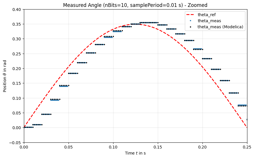
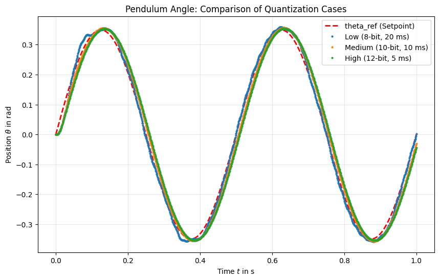
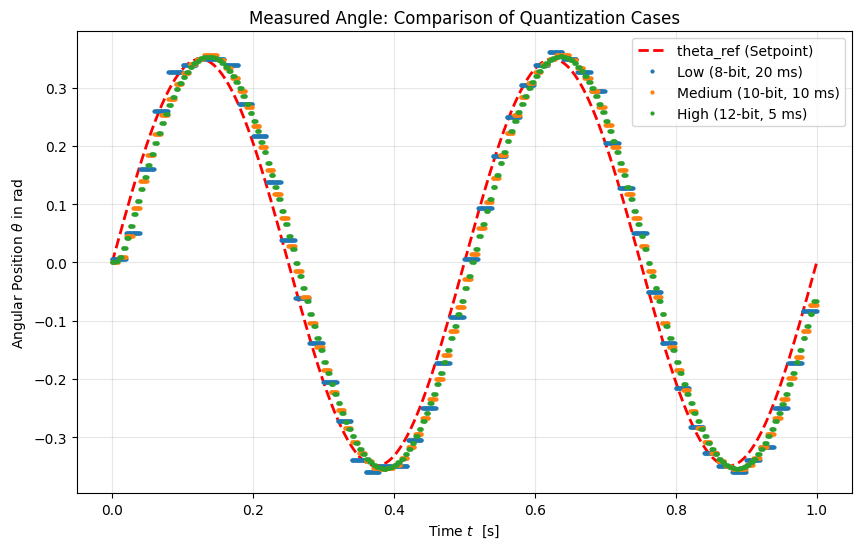
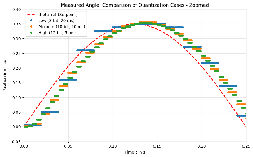
3.16. Plot: Decoder Outputs#

This plot shows how sampling and quantization affect the decoded angle.

Hide code cell source

plt.figure(figsize=(10, 6))
plt.plot(t_setpoint, theta_ref, label="theta_ref (Setpoint)", color='red', linestyle='--', linewidth=2)
plt.plot(case_low['t_pendulum'], case_low['theta_pendulum'], 'o', label=case_low['label'], markersize=2)
plt.plot(t_pendulum, theta_pendulum, 'o', label="Medium (10-bit, 10 ms)", markersize=2)
plt.plot(case_high['t_pendulum'], case_high['theta_pendulum'], 'o', label=case_high['label'], markersize=2)
plt.xlabel(r"Time $t$  [s]")
plt.ylabel(r"Angular Position $\theta$  [rad]")
plt.title(f"Pendulum Angle: Comparison of Quantization Cases")
plt.legend()
plt.grid(True, alpha=0.3)
plt.show()
../_images/6f2dc02b8a41478d5455ed5afc867d655cb29557cd0c9121584a987231b78c3e.png

Hide code cell source

plt.figure(figsize=(10, 6))
plt.plot(t_setpoint, theta_ref, label="theta_ref (Setpoint)", color='red', linestyle='--', linewidth=2)
plt.plot(case_low['t_dec'], case_low['theta_dec'], 'o', label=case_low['label'], markersize=2)
plt.plot(t_decoder, theta_decoder, 'o', label="Medium (10-bit, 10 ms)", markersize=2)
plt.plot(case_high['t_dec'], case_high['theta_dec'], 'o', label=case_high['label'], markersize=2)
plt.xlabel(r"Time $t$  [s]")
plt.ylabel(r"Angular Position $\theta$  [rad]")
plt.title(f"Measured Angle: Comparison of Quantization Cases")
plt.legend()
plt.grid(True, alpha=0.3)
plt.show()
../_images/ede81b9bb710b7019d7f5624a1291ca7b45036a02f22d0a25e32c0387f57e1cf.png

Hide code cell source

plt.figure(figsize=(10, 6))
plt.plot(t_setpoint, theta_ref, label="theta_ref (Setpoint)", color='red', linestyle='--', linewidth=2)
plt.plot(case_low['t_dec'], case_low['theta_dec'], 'o', label=case_low['label'], markersize=2)
plt.plot(t_decoder, theta_decoder, 'o', label="Medium (10-bit, 10 ms)", markersize=2)
plt.plot(case_high['t_dec'], case_high['theta_dec'], 'o', label=case_high['label'], markersize=2)
plt.xlim(0, 0.5)
plt.ylim(-0.05, 0.4)
plt.xlabel(r"Time $t$  [s]")
plt.ylabel(r"Angular Position $\theta$  [rad]")
plt.title(f"Measured Angle: Comparison of Quantization Cases - Zoomed")
plt.legend()
plt.grid(True, alpha=0.3)
plt.show()
../_images/71b7af92d23d1df93adfa738a76b40fc40bdd8c4736271ddf64661780cfa4980.png

3.17. Summary#

  • Higher resolution and faster sampling reduce quantization artifacts in theta_meas.

  • Control performance degrades at low resolution and slow sampling.