

1. FEM Pendulum: Basics#
In this FEM tutorial section, we will build a deformable pendulum model using the Finite Element Method (FEM) with NGSolve.
Basics (this tutorial): We set up the basic model of a deformable pendulum without contact and external torque.
Torque Application: We extend the basic model by applying an external torque at the pivot point.
Contact Handling: We further extend the model by adding contact handling with a wall.
Following references were used to implement the model:
FEM pendulum swing.#
1.1. Overview#
We construct a planar pendulum from scratch:
geometry,
mesh,
material law,
mixed FE space with hinge constraint,
nonlinear energy, and
a Newmark time integrator.
This notebook focuses on the core mechanics before adding torque actuation or wall contact.
1.2. Learning Goals#
Build a 2D pendulum mesh with labeled boundaries
Define a Neo-Hookean material model (hyperelasticity)
Set up mixed FE spaces with a hinge constraint using
NumberSpaceAssemble the nonlinear weak form (internal forces + inertia + gravity + constraints)
Time-integrate by solving the nonlinear weak form with Newton’s method (NGSolve:
NewtonMinimization) and Newmark-style updatesExtract a rigid-body proxy angle from the deformable solution
1.3. Prerequisites and Setup#
You should be comfortable with basic FEM ideas (weak form, trial/test spaces) and nonlinear elasticity. The notebook uses NGSolve + Netgen. All quantities are in SI units.
Assumptions used here:
2D planar model with an out-of-plane thickness
Hyperelastic (Neo-Hookean) material
No damping, no contact, no external torque
Documentation note: The NGSolve Draw(...) scenes are ipywidgets-based. To get the interactive WebGUI scenes in the rendered HTML docs, run this notebook once and save the widget state (JupyterLab: Command Palette → “Save Notebook Widget State”) before building the docs.
import matplotlib.pyplot as plt
import numpy as np

from netgen.occ import *
from ngsolve import *
from ngsolve.solvers import NewtonMinimization
from ngsolve.webgui import Draw
1.4. Physical Model and Governing Equation#
We model a deformable pendulum in 2D (with a constant out-of-plane thickness) using a displacement field \(u(X,t)\).
A standard nonlinear elastodynamics form in the reference configuration is:
where
\(\rho_0\) is the reference density (here: \(\rho_0 = \rho\, t\) for 2D-thickness scaling),
\(P\) is the first Piola-Kirchhoff stress,
\(b\) is a body force (gravity).
In a hyperelastic model, internal forces come from a strain energy density \(W(F)\) with
We do not assemble a single global stiffness matrix once. Instead, we solve the nonlinear weak form at each time step using Newton iterations (residual + linearization).
1.5. Material Law#
We use a Neo-Hookean hyperelastic model. This is suitable for large deformations and avoids the limitations of linear elasticity for large rotations.
1.5.1. Dimensional reduction: 2D plane stress#
The pendulum is three-dimensional, but we reduce to a 2D planar model for reduced computational cost. The reduction is consistent under a plane-stress assumption, which is appropriate for a thin body with \(\sigma_{zz} = 0\) (free out-of-plane surfaces). This will be applied consistently throughout the tutorial series: the pendulum thickness is small, mass is scaled by thickness, and the constitutive law uses plane-stress-adjusted Lamé parameters.
Under plane stress, the out-of-plane stress \(\sigma_{zz}\) is eliminated statically, which modifies the first Lamé parameter:
The shear modulus \(\mu\) is unchanged. Using \(\lambda^{*}\) in the 2D strain energy yields the correct plane-stress response at small strains and a consistent finite-strain extension.
1.5.2. Material Parameters#
We specify Young’s modulus and Poisson’s ratio, then compute the plane-stress Lamé parameters.
E = 2.1e11      # Young's modulus in Pa
nu = 0.3        # Poisson's ratio

# Plane-stress Lamé parameters (σ_zz = 0)
lam = E * nu / (1 - nu * nu)
mu = E / (2 * (1 + nu))
1.5.3. Deformation Gradient#
The deformation gradient is \(F\), and the right Cauchy-Green tensor is \(C\) are defined as:
def C(u):
    F = Id(2) + Grad(u)
    return F.trans * F
1.5.4. Hyperelastic Material Strain Energy Density Function#
We use the Neo-Hookean strain energy density function:
def psi(C, lam, mu):
    return (mu / 2) * (Trace(C - Id(2)) + (2 * mu / lam) * (Det(C))**(-lam / (2 * mu)) - 1)
1.5.5. Stress Tensors (for post-processing)#
The 2nd Piola-Kirchhoff stress is derived from the strain energy density:
For the Neo-Hookean energy, differentiating with respect to \(C\) gives
For a meaningful visualization we push \(S\) forward to the Cauchy (true) stress in the current configuration:
Under the plane-stress assumption (\(\sigma_{zz} = \sigma_{xz} = \sigma_{yz} = 0\)), the von Mises equivalent stress reduces to
Note: In the time-stepping loop we use the energy-based
Variation(...)approach, which lets NGSolve derive residual and tangent automatically. The explicit stress expressions below are provided for post-processing only and are not called during the solve.
def PK2_neo_hookean(u, lam, mu):
    """2nd Piola-Kirchhoff stress for the Neo-Hookean model.

    S = mu * (I - det(C)^(-lam/(2*mu)) * C^{-1})
    """
    CC = C(u)
    return mu * (Id(2) - Det(CC)**(-lam / (2 * mu)) * Inv(CC))

def cauchy_stress(u, lam, mu):
    """Cauchy (true) stress: sigma = (1/J) F S F^T."""
    F = Id(2) + Grad(u)
    J = Det(F)
    S = PK2_neo_hookean(u, lam, mu)
    return (1 / J) * F * S * F.trans

def von_mises(u, lam, mu):
    """Plane-stress von Mises: sigma_vM = sqrt(sxx^2 + syy^2 - sxx*syy + 3*sxy^2)."""
    sigma = cauchy_stress(u, lam, mu)
    sxx, syy, sxy = sigma[0, 0], sigma[1, 1], sigma[0, 1]
    return sqrt(sxx * sxx + syy * syy - sxx * syy + 3 * sxy * sxy)
1.6. Create Geometry and Mesh#
We define a simple pendulum: a rectangular rod with a circular head and a hole. The top edge is labeled as the rotation (hinge) boundary.
1.6.1. Geometry Parameters#
Key geometric parameters (meters):
r_rod: half-width of the rodr_head: radius of the pendulum headr_hole: hole radius (subtracted)l_center: length from pivot to head center
r_rod = 0.015   # rod radius in meters
r_hole = 0.03   # hole radius in meters
r_head = 0.06   # head radius in meters
l_center = 0.24 # length to center of head in meters
1.7. Create Geometry#
1.7.1. Named Regions and Integration Measures#
In Netgen/NGSolve we can name materials (faces) and boundaries (edges). These names show up in the integration measures:
dx("pendulum"): integrate over the material region namedpendulumds("rotation"): integrate over the boundary namedrotation
This is how we keep the weak form readable and ensure each term is integrated on the correct part of the domain.
bar = MoveTo(-r_rod, 0).Rectangle(2 * r_rod, l_center).Face()
bar.edges.Min(Y).name = "rotation"
bar.edges.Min(Y).maxh = r_rod / 10
bar.faces.name = "bar"
bar.faces.maxh = r_rod / 2

hole = Circle((0, l_center), r_hole).Face()
hole.faces.name = "hole"
hole.edges.maxh = r_head / 20

circ = Circle((0, l_center), r_head).Face()
circ.edges.maxh = r_head / 20
circ.faces.name = "circ"
circ.faces.maxh = r_head / 5
circ.edges.name = "contact_head"

head = circ - hole
pendulum = head + bar - hole

pendulum = pendulum.Rotate(Axis((0.0, 0, 0), (0, 0, 1)), 180)
pendulum.name = "pendulum"

# Refine min y vertices on edge 0 and edge 1
pendulum.vertices[0].maxh = r_rod / 20
pendulum.vertices[1].maxh = r_rod / 20
1.7.2. Generate Mesh#
We generate a curved, quadratic mesh for better geometric accuracy of the circular head.
geo = OCCGeometry(pendulum, dim=2)

max_element_size = 0.03
mesh_order = 2

mesh = Mesh(geo.GenerateMesh(maxh=max_element_size))
mesh.Curve(mesh_order)

scene_mesh = Draw(mesh)
print(f"Number of elements in the mesh: {mesh.ne}")
print(f"Number of vertices in the mesh: {mesh.nv}")
Number of elements in the mesh: 1180
Number of vertices in the mesh: 712
1.8. Initialize FE Spaces#
1.8.1. Hinge Constraint#
Without constraints, a free elastic body under gravity would translate and fall. A pendulum needs a pivot that prevents translation at the top while still allowing rotation.
In this tutorial we enforce a mean-zero displacement constraint on the top edge rotation using Lagrange multipliers. This is a common, robust approximation of a hinge in FEM.
1.8.2. Mixed space#
We use a mixed space to enforce the hinge constraint:
\(V = [H^1(\Omega_0)]^2\) for displacement
\(Q = \mathrm{NumberSpace}\) on the rotation boundary
rotationMixed space: \(V \times Q^2\) (two multipliers for x and y constraints)
Because functions in NumberSpace are constant on the chosen boundary, the constraint effectively enforces
This removes rigid translation of the hinge edge while leaving rotation free.
V = VectorH1(mesh, order=2)
Q = NumberSpace(mesh, definedon=mesh.Boundaries("rotation"))
Trial and Test Functions:
Displacement Trial function:
\[u \in V\]Displacement Test function:
\[v \in V\]Scalar Lagrange Multipliers \(q\) and \(p\) living on the rotation boundary:
\[q, p \in Q²\]
FES = V * Q**2
(u, q), (v, p) = FES.TnT()

# Post-processing spaces on the pendulum material
S_sigma = MatrixValued(H1(mesh, order=2, definedon=mesh.Materials("pendulum")))  # Cauchy tensor
S_vm    = H1(mesh, order=2, definedon=mesh.Materials("pendulum"))                # von Mises scalar

# Current grid functions
gf_u = GridFunction(FES)
gf_v = GridFunction(FES)
gf_a = GridFunction(FES)

# Previous time step grid functions
gf_u_old = GridFunction(FES)
gf_v_old = GridFunction(FES)
gf_a_old = GridFunction(FES)

# Stress grid functions (for post-processing)
gf_sigma = GridFunction(S_sigma)  # Cauchy stress tensor
gf_vm    = GridFunction(S_vm)     # von Mises scalar

# History grid functions for post-processing
gf_u_history  = GridFunction(V, multidim=0)
gf_v_history  = GridFunction(V, multidim=0)
gf_a_history  = GridFunction(V, multidim=0)
gf_vm_history = GridFunction(S_vm, multidim=0)
1.9. Setup the Bilinear Form#
We assemble a nonlinear weak form \(R(w) = 0\) on the mixed space \(w = (u,q)\).
Conceptually (schematic), the contributions are:
internal forces from hyperelasticity (nonlinear in \(u\))
inertial forces via Newmark-style time discretization (depends on \(u\) and previous states)
body force (gravity)
hinge constraint terms coupling \(u\) and the Lagrange multipliers
In NGSolve, BilinearForm can represent nonlinear operators. For hyperelasticity we add an energy density and wrap it in Variation(...) so NGSolve can automatically generate:
the residual vector \(R(w)\), and
the linearization (tangent) needed by Newton.
Other terms (constraint, inertia, gravity) are added directly in weak form notation using dx("pendulum") and ds("rotation").
bfa = BilinearForm(FES)
1.9.1. Strain Energy of the Pendulum#
This term encodes internal elastic forces via the hyperelastic strain energy density \(W(F)\).
In code we integrate the energy density over the pendulum domain and wrap it in Variation(...):
Variation(W(u) * dx)tells NGSolve to treat the expression as a nonlinear functional.NGSolve then computes the residual (first variation) and the linearization (tangent) needed by Newton’s method.
bfa += Variation(psi(C(u), lam, mu) * dx("pendulum"))
1.9.2. Rotation Constraint#
We enforce a hinge by constraining the average displacement on the top edge rotation to zero.
Using Lagrange multipliers (two scalars for x and y) yields the saddle-point coupling
This removes rigid translation of the rotation edge while allowing the pendulum to rotate freely.
bfa += (InnerProduct(u, p) + InnerProduct(v, q)) * ds("rotation")
1.9.3. Inertial Term (Newmark)#
We model dynamics by including the inertial term
and expressing the new acceleration \(a^{n+1}\) from the unknown displacement \(u^{n+1}\) and the stored previous states \((u^n, v^n, a^n)\) via Newmark-style updates:
In this basic tutorial we add this term directly in weak form notation (it is linear in the test function \(v\) and depends on \(u\) through the update formulas).
tau = Parameter(0.01)

vel_new = 2/tau * (u - gf_u_old.components[0]) - gf_v_old.components[0]

acc_new = 2/tau * (vel_new - gf_v_old.components[0]) - gf_a_old.components[0]

thickness = 0.01 # thin plate (plane-stress assumption), in meters
rho = 7800       # density in kg/m^3

bfa += rho * thickness * InnerProduct(acc_new, v) * dx("pendulum")
1.9.4. Gravitational Force#
Gravity acts in negative y-direction.
In weak form we include the body force contribution as
with \(e_y=(0,1)\) and \(g>0\) (magnitude). In code we build an explicit gravity vector pointing downward.
g = 9.81  # gravity magnitude in m/s^2
# gravity vector points downward (negative y)
gvec = CF((0, -g))

# Body force term in the residual: -\int rho*t*gvec · v dx
bfa += -rho * thickness * InnerProduct(gvec, v) * dx("pendulum")
1.10. Set Initial State#
We initialize the pendulum by applying a rigid-body rotation to the reference coordinates and set the initial displacement field accordingly.
theta0 = np.deg2rad(20)  # initial angle in radians
omega0 = 0.0             # initial angular velocity in rad/s

# Coordinates of pivot point
x_pivot = 0
y_pivot = 0

# relative position vector from pivot to point in pendulum
r = CF((x - x_pivot, y - y_pivot))

c, s = np.cos(theta0), np.sin(theta0)

r0 = CF((c * r[0] - s * r[1],
         s * r[0] + c * r[1]))
u0 = CF((r0[0] - r[0],
         r0[1] - r[1]))
gf_u.components[0].Set(u0, definedon=mesh.Materials("pendulum"))
gf_u_old.components[0].Set(u0, definedon=mesh.Materials("pendulum"))

scene = Draw(gf_u.components[0],
             mesh,
             "Displacement",
             deformation=gf_u.components[0],
             show=True,
)
1.10.1. Rigid Body Approximation#
We estimate the pendulum angle from the deformable displacement field by projecting onto a rigid rotation. This is a proxy, not an exact kinematic constraint.
def rigid_body_proxy(gf_u):
    u = gf_u.components[0]

    denom = Integrate(InnerProduct(r, r), mesh, definedon=mesh.Materials("pendulum"))

    s_num = Integrate(r[0] * u[1] - r[1] * u[0], mesh, definedon=mesh.Materials("pendulum"))
    c_num = Integrate(InnerProduct(r, r + u), mesh, definedon=mesh.Materials("pendulum"))

    s = s_num / denom
    c = c_num / denom

    theta = np.arctan2(s, c)

    return theta
theta_applied = rigid_body_proxy(gf_u)
print(f"Initial angle from rigid body proxy: {np.rad2deg(theta_applied):.2f} degrees")
Initial angle from rigid body proxy: 20.00 degrees
1.11. Time Stepping Loop#
At each time step we solve the nonlinear weak form with Newton iterations using NGSolve’s NewtonMinimization helper (it computes residual and linearization from the assembled BilinearForm).
After the solve, we update velocity and acceleration using the Newmark-style formulas and store the displacement history for plotting/animation.
t = 0.0
t_end = 1.0

t_vals = []
theta_vals = []

dt = tau.Get()
n_steps = int(t_end / dt)
for step in range(n_steps):
    gf_u_old.vec[:] = gf_u.vec
    gf_v_old.vec[:] = gf_v.vec
    gf_a_old.vec[:] = gf_a.vec

    NewtonMinimization(
        a=bfa,
        u=gf_u,
        printing=False,
        inverse="sparsecholesky",
        maxerr=1e-6,
        maxit=20,
    )

    theta_current = rigid_body_proxy(gf_u)
    t_vals.append(t)
    theta_vals.append(theta_current)

    gf_v.vec[:] = 2/tau.Get() * (gf_u.vec - gf_u_old.vec) - gf_v_old.vec
    gf_a.vec[:] = 2/tau.Get() * (gf_v.vec - gf_v_old.vec) - gf_a_old.vec

    # Post-processing: Cauchy stress tensor and plane-stress von Mises scalar
    u_cur = gf_u.components[0]
    gf_sigma.Interpolate(cauchy_stress(u_cur, lam, mu))
    gf_vm.Set(von_mises(u_cur, lam, mu))

    gf_u_history.AddMultiDimComponent(gf_u.components[0].vec)
    gf_v_history.AddMultiDimComponent(gf_v.components[0].vec)
    gf_a_history.AddMultiDimComponent(gf_a.components[0].vec)
    gf_vm_history.AddMultiDimComponent(gf_vm.vec)

    t += tau.Get()
    print(f"Time step {step+1}/{n_steps}, time={t:.4f} s", end="\r")
Time step 100/100, time=1.0000 s
settings = {"Multidim": {"speed": 15}}

def animate(gf_hist, settings=settings):
    Draw(
        gf_hist,
        mesh,
        interpolation_multidim=True,
        deformation=gf_hist,
        animate=True,
        autoscale=True,
        settings=settings,
    )

def animate_stress(gf_sigma_hist, gf_u_hist, settings=settings):
    Draw(
        gf_sigma_hist,
        mesh,
        interpolation_multidim=True,
        deformation=gf_u_hist,
        animate=True,
        autoscale=False,
        min=0,
        max=np.max([v.FV().NumPy().max() for v in gf_sigma_hist.vecs]),
        settings=settings,
    )
animate(gf_u_history, settings=settings)
The above animation shows the displacement field evolving over time. The displacement is minimal in the vertical position of the pendulum and maximal at the turning points.
1.11.1. Von Mises Stress Animation#
The following animation shows the plane-stress von Mises equivalent stress \(\sigma_{\mathrm{vM}}\) (computed from the Cauchy stress \(\sigma\)) on the deformed configuration. Stress concentrations are visible at the hinge (pivot edge) and at the rod–head junction.
animate_stress(gf_vm_history, gf_u_history, settings=settings)
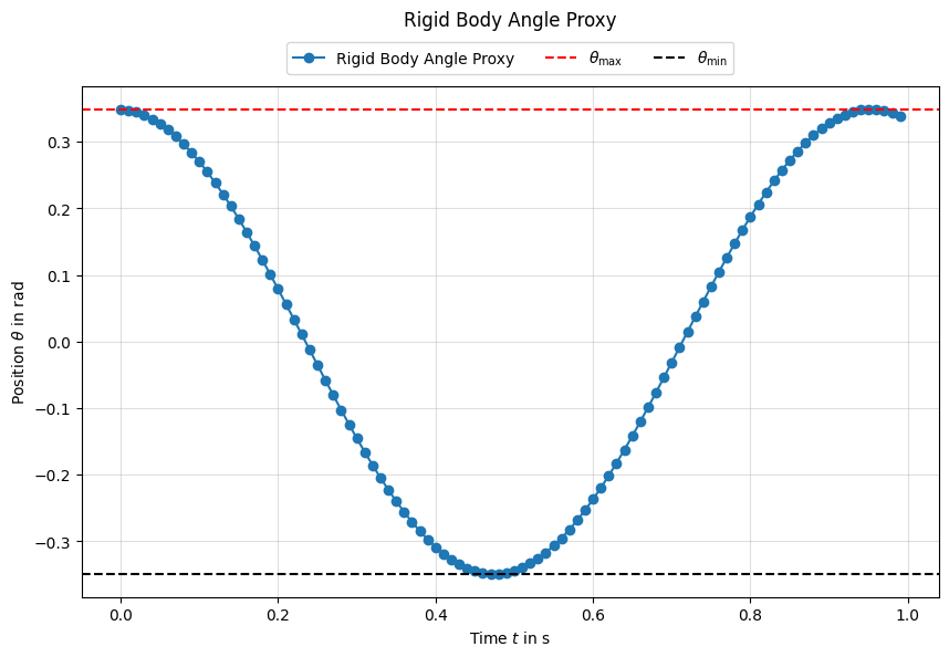
1.12. Plot Trajectory#
We can also plot the estimated rigid-body angle over time to visualize the pendulum swing. The angle is extracted by projecting the deformable solution onto a rigid rotation, so it is a proxy for the actual pendulum angle.
1.13. Conclusion#
This tutorial demonstrated how to build a basic deformable pendulum model using the Finite Element Method with NGSolve.
We covered:
geometry and mesh creation with named regions
defining a Neo-Hookean hyperelastic material
setting up a mixed FE space with a hinge constraint using
NumberSpaceassembling the nonlinear weak form (internal forces + inertia + gravity + constraints)
time-integrating by solving the nonlinear weak form with Newton’s method (NGSolve:
NewtonMinimization) and Newmark-style updatesextracting a rigid-body proxy angle from the deformable solution