3. Concepts

This page introduces the core ideas behind SysSimX. It builds a mental model in layers: first why co-simulation is needed, then the building blocks (components, ports, connections), and finally how SysSimX orchestrates them in time (execution order, algebraic loops, master algorithms, and events).

If you just want to run your first simulation, start with the Quickstart and come back here when you want to understand what happens under the hood.

3.1. Why Co-Simulation?

Realistic engineering systems are heterogeneous: a controller may be designed in Modelica and exported as an FMU, a structure may be modeled with finite elements, and human motion may come from a musculoskeletal model. No single tool covers all of these domains well.

Co-simulation couples such subsystems while each keeps its own solver. Every subsystem advances itself internally and only exchanges input/output signals with the others at discrete points in time:

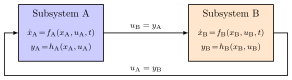
Data is exchanged on a communication grid: the macro step \(H_k\) is the interval between two communication points \(T_k\) and \(T_{k+1}\), while each subsystem may internally take several smaller micro steps \(\Delta t\) with its own solver:

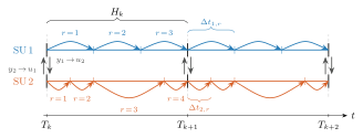
Between communication points, each subsystem extrapolates (holds) its inputs. This decoupling is what makes it possible to combine tools — but it also introduces the coordination questions (ordering, loops, events) that the rest of this page is about.

3.2. The Big Picture

SysSimX is a Python framework that acts as the master of such a co-simulation: it owns the components, resolves their coupling, and advances them consistently in time. The framework is organized in four layers between your user code and the external simulation tools:

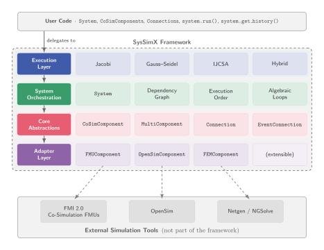
• Adapter layer — wraps external tools (FMUs, OpenSim, NGSolve) behind one uniform component interface. New tools are integrated by writing a new adapter.

• Core abstractions — CoSimComponent, MultiComponent, Connection, and EventConnection: the vocabulary you use to describe a system.

• System orchestration — the System container analyzes the coupling structure (dependency graph, execution order, algebraic loops).

• Execution layer — the master algorithms (Jacobi, Gauss–Seidel, IJCSA, Hybrid) that actually advance the system in time.

As a user you mostly interact with the top: create components, connect them, call system.run(), and read back results with system.get_history().

3.3. Mental Model: System, Component, Connection

Four terms are enough to describe any SysSimX model:

Concept	Meaning
Component	A model with input ports u, output ports y, parameters, and (optionally) internal state.
Connection	A directed signal path from an output port to an input port.
System	The container that owns components and connections and orchestrates execution.
Step	One advance of the whole system by a macro step dt.

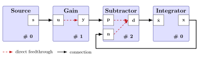
The figure below shows a small system of four components. Solid arrows are connections between ports; red dashed arrows inside a component mark direct feedthrough (the output depends on the input at the same instant); blue dashed arrows are event connections carrying discrete events instead of continuous signals:

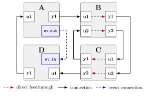
In code, the same structure reads almost like the picture:

system = System("example")
system.add_component(a)
system.add_component(b)
system.connect(a, "y1", b, "u1")   # output port -> input port
system.run(t_end=10.0, dt=0.01)

3.4. Components

Every model in SysSimX — whether it wraps an FMU, a finite element solver, or ten lines of Python — implements the same abstract base class CoSimComponent. The base class defines the typed port interface, the lifecycle, and a set of optional capabilities (dashed borders below) that the master algorithms can exploit when present:

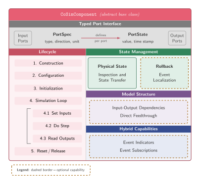
• Lifecycle — construction, configuration, initialization, the simulation loop, and reset/release (details below).

• State management — components may expose their physical state for inspection or support rollback, which the hybrid algorithm uses to localize events precisely.

• Model structure — components declare their input–output dependencies (direct feedthrough), which drives the execution-order analysis.

• Hybrid capabilities — components may publish event indicators or subscribe to events from others.

Built-in adapters exist for common tools, and custom components are plain Python classes:

Component	Wraps
FMUComponent	FMI 2.0 Co-Simulation FMUs
FEMComponent	NGSolve-based finite element models
OpenSimComponent	OpenSim musculoskeletal models
custom CoSimComponent subclass	any Python code

3.4.1. The Simulation Step

During the simulation loop, each macro step of a component follows a fixed pattern: the algorithm sets the inputs, calls do_step(t, dt), and reads the outputs. Inside do_step, the base class delegates the tool-specific work to two abstract hooks and takes care of time bookkeeping and result recording itself:

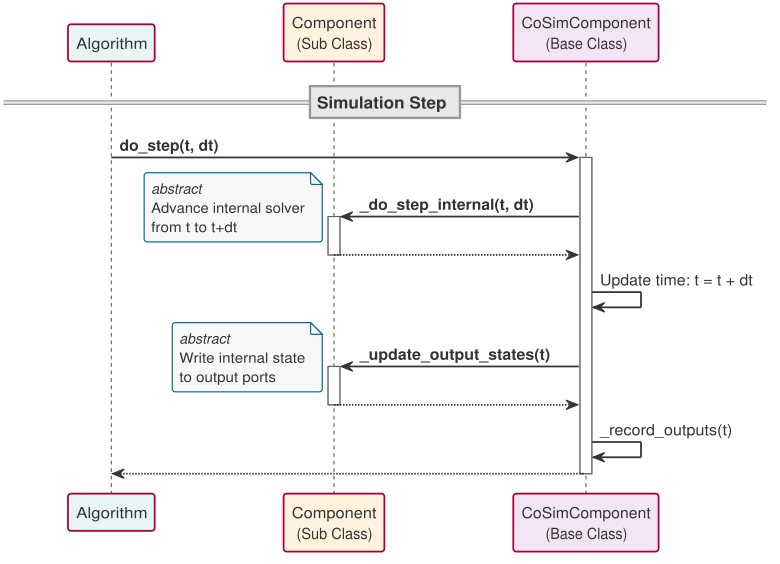
This split is what makes adapters small: a new component only implements advance the internal solver and write internal state to the output ports — everything else (port handling, unit conversion, history recording) is inherited.

After (or during) a run you retrieve results with component.get_outputs() for the current values or system.get_history() for the full recorded time series.

3.5. Ports and Units

Ports are the interface of a component. Each port separates an immutable contract (PortSpec: name, type, direction, optional unit) from its mutable runtime state (PortState: current value and timestamp):

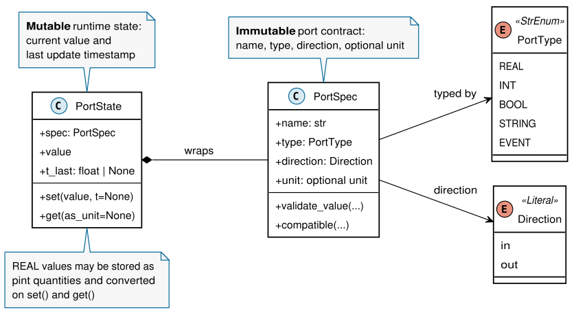
Two consequences matter in practice:

1. Type safety — a connection is only valid if the two port specs are compatible (matching type, out → in direction). Mistakes are caught at connect time, not as silent numerical errors during the run.

2. Automatic unit conversion — units are handled with Pint. If a drive outputs torque in N*m and a biomechanics model expects N*mm, the connection converts automatically. This is essential when combining tools with different unit conventions.

3.6. Execution Order and Direct Feedthrough

Before the first step, the System performs a structural analysis of the coupling. Components and connections form a directed dependency graph; a connection into a direct-feedthrough input is a zero-delay edge, because the downstream output needs the upstream value at the same instant:

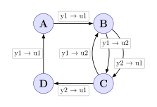
From this graph SysSimX derives a generation-based execution order: components in the same generation have no zero-delay dependency on each other and can be evaluated together (even in parallel); later generations run after the components that feed them. Components whose outputs only depend on their internal state (no feedthrough) break the chain and can be scheduled freely:

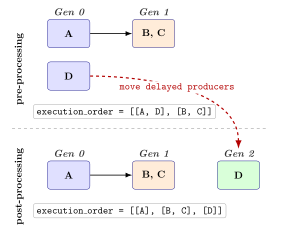
You never specify this order manually — it is recomputed automatically whenever the topology changes.

3.7. Algebraic Loops

If zero-delay (direct-feedthrough) edges form a cycle, no valid ordering exists: each component needs the other’s output first. This is an algebraic loop. During structural analysis, SysSimX detects these cycles as strongly connected components (SCCs) of the zero-delay graph:

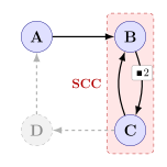
Loops are not an error — they are solved iteratively at each communication point using the IJCSA method (Interface Jacobian-based Co-Simulation Algorithm): the loop components are evaluated repeatedly, with a Newton-type update on the interface variables, until the coupling residual converges. Everything outside the loop still runs in the normal generation order.

3.8. Master Algorithms

The master algorithm decides when each component steps and which input values it sees. SysSimX provides two classic schemes for continuous coupling:

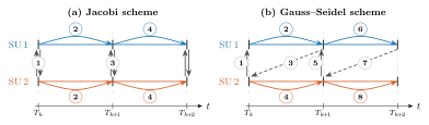
• Jacobi — all components step in parallel using the input values from the previous communication point. Fast and parallelizable, but feedthrough signals effectively lag by one macro step.

• Gauss–Seidel — components step sequentially in execution order, so downstream components already see the current values of their upstream neighbors. More accurate for feedthrough chains, at the cost of sequential execution.

In addition:

• IJCSA — iterative solver used for systems with algebraic loops (see above).

• Hybrid — event-driven stepping with zero-crossing localization (see below).

You normally don’t choose the algorithm yourself: the System selects the appropriate one from the structural analysis (loops present? event sources present? feedthrough chains?). The accuracy difference is visible in a simple feedthrough benchmark — Jacobi shows the characteristic one-step lag at large step sizes, while Gauss–Seidel and IJCSA stay close to the analytic solution; with decreasing macro step size all schemes converge:

3.9. Multi-Model Components

Often the right model fidelity depends on the operating condition: a rigid-body pendulum is cheap and accurate in free swing, but a finite element model is needed near contact. A MultiComponent bundles several models of the same physical subsystem behind one unified port interface and switches between them at runtime:

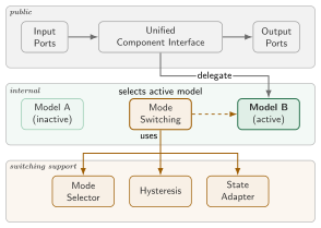
• A mode selector decides which model should be active (e.g., based on distance to contact).

• Hysteresis prevents rapid back-and-forth switching at the decision boundary.

• A state adapter transfers the physical state from the deactivated model to the newly activated one, so the switch is continuous.

From the outside, the rest of the system never notices the switch — the MultiComponent looks like any other component.

3.10. Events and Hybrid Simulation

Many systems are hybrid: continuous dynamics interrupted by discrete events — a contact, a switch, an impact. At an event time \(t_i\), a continuous state may jump (\(x^- \to x^+\), e.g., a velocity reversal at impact) and a discrete mode may change (\(q^- \to q^+\)):

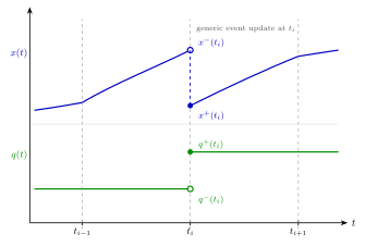
Handling this accurately in a co-simulation requires more than fixed steps. The hybrid master algorithm localizes each event by bisection, illustrated below for a pendulum hitting a wall (event indicator \(\gamma(t) = \theta(t) - \theta_{\mathrm{wall}}\), ideal elastic impact):

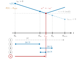
1. Detect — a trial step \(T_k \to T_{k+1}\) shows a sign change of the indicator (\(\gamma_k > 0\), \(\gamma_{k+1} < 0\)): an event lies inside the step. The components are rolled back to their snapshots at \(T_k\).

2. Bisect — a trial step over the left half \([T_k, T_m]\) shows no crossing (\(\gamma_m > 0\)), so the event must lie in the right half.

3. Refine — stepping continues from \(T_m\) with halved intervals (\(\Delta t/4\), \(\Delta t/8\), …), keeping whichever half brackets the crossing, until the event time \(t_{\mathrm{ev}}\) is located within tolerance.

4. Commit — the components are restored once more and take one accepted step exactly to \(t_{\mathrm{ev}}\); event handlers are dispatched at that dense time (here the impact handler \(\omega^+ = -\omega^-\)) and subscribed components are notified via event connections. Continuous stepping then resumes from \(t_{\mathrm{ev}}\).

This is why the rollback capability from the component capability map matters: without snapshots, trial steps could not be discarded.

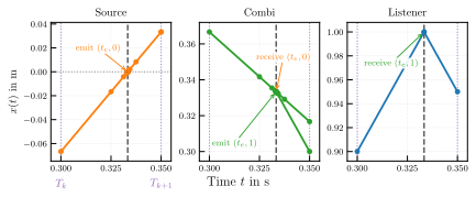
Events can also cascade: one component’s event changes another component’s inputs, which may immediately trigger a follow-up event at the same instant. SysSimX processes such event chains to completion before continuous time resumes:

3.11. Putting It All Together

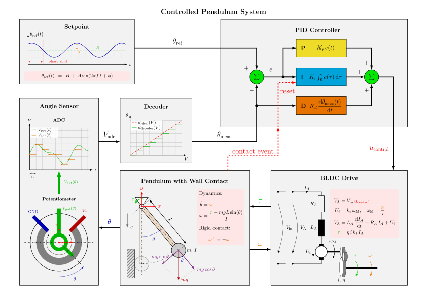
The controlled pendulum below combines everything from this page in one system: a setpoint source, a PID controller, a BLDC drive, a pendulum with wall contact, and a sensor chain (potentiometer → ADC → decoder) closing the feedback loop. The wall contact is a discrete event that reverses the angular velocity and resets the controller’s integrator via an event connection:

Reading it with the concepts from this page:

• Each block is a component with typed, unit-aware ports; the arrows are connections.

• The controller and sensor chain have direct feedthrough, so the execution order matters within each step.

• The closed control loop is broken by the pendulum’s internal state — no algebraic loop remains.

• The wall contact is a zero-crossing event; the dashed red contact event line is an event connection that resets the PID integrator.

• The pendulum itself can be a multi-model component, switching between a cheap rigid-body model in free swing and an FEM model near contact.

This system is developed step by step in the controlled pendulum case study and its linked notebooks.

3.12. Where to Go Next

• Quickstart — build and run your first system in a few lines.

• Core tutorials — build systems from simple components to hybrid simulations.

• Controlled pendulum case study — follow the complete multi-stage example.

• SysSimX package API and component API — reference documentation for the framework.