

2. Modelica Pendulum: Discrete Contact#
This tutorial extends the basic pendulum model to a discrete wall-contact case and analyzes state-event behavior after FMU export.
The main objective is to show a practical co-simulation fact: for FMUs that contain Modelica state events, the detected event instant at the master level is sensitive to the macro communication step size dt.
2.1. Overview#
We will:
Define a Modelica pendulum with discrete impact (
when+reinit).Compute a direct Modelica reference trajectory (
dassl).Export FMI 2.0 co-simulation FMUs (
cvode,euler).Run FMUs in
syssimxwith different macro step sizes.Compare first-contact timing and penetration indicators.
This isolates macro-step sensitivity before introducing hybrid rollback algorithms.
2.2. Learning Goals#
Understand how Modelica expresses impact events through equation-level state events.
Understand why FMU co-simulation exposes event timing only at communication boundaries.
Quantify how reducing macro step size improves observed event-time accuracy.
Prepare the foundation for the next tutorials on rollback-based event localization and explicit event handling in
syssimx.
2.3. Prerequisites and Setup#
We assume the setup from tutorial 01 is available:
OpenModelica +
OMPythonsyssimxPython environmentplotting stack (
numpy,matplotlib)
The model used here is PendulumDiscreteContact.mo.
import numpy as np
import matplotlib.pyplot as plt

from OMPython import ModelicaSystem
from syssimx import FMUComponent
2.4. Theory: Discrete Contact in Modelica#
For the pendulum state
a rigid wall at theta_wall is represented as a state event:
event condition:
theta <= theta_wallevent action:
reinit(omega, -omega)(ideal elastic velocity inversion)
In direct Modelica simulation, variable-step solvers (e.g., dassl) localize event times internally with root-finding.
In FMI 2.0 co-simulation, the master advances the FMU by macro steps (do_step(t, dt)), and outputs are observed at communication points. Therefore, coarse dt can delay detected event instant, while smaller dt generally increases temporal accuracy at higher computational cost.
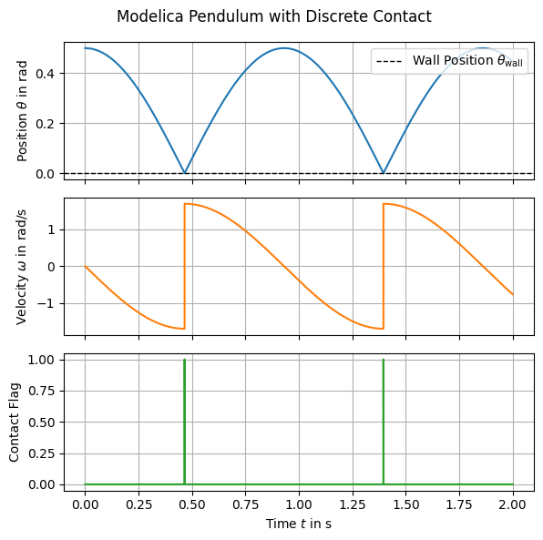
2.5. Modelica Implementation#
The model below contains:
continuous pendulum dynamics (
theta,omega)discrete impact handling with
when/reinita Boolean
contactoutput for diagnostics
This contact signal is useful to compare event observability between direct Modelica simulation and FMU co-simulation.
model PendulumDiscreteContact
  // Imports
  import Modelica.Constants.pi;

  // Parameters
  parameter Real m(unit="kg") = 40;
  parameter Real L(unit="m") = 0.6;
  parameter Real theta0(unit="rad") = 0;
  parameter Real omega0(unit="rad/s") = 0;
  parameter Real g(unit="m/s2") = 9.81;
  parameter Real inertia(unit="kg.m2") = 20;
  parameter Real theta_wall (unit="rad") = 0;
  parameter Integer sense = -1;

  // Input torque at the pivot
  Modelica.Blocks.Interfaces.RealInput torque(unit="N.m");

  // Outputs
  Modelica.Blocks.Interfaces.RealOutput theta(unit="rad");
  Modelica.Blocks.Interfaces.RealOutput omega(unit="rad/s");
  Modelica.Blocks.Interfaces.RealOutput alpha(unit="rad/s2") = der(omega);
  Modelica.Blocks.Interfaces.BooleanOutput contact;

initial equation
  theta = theta0;
  omega = omega0;
  contact = theta <= theta_wall and omega < 0;

equation
  der(theta) = omega;
  der(omega) = -(m * g * L / inertia) * sin(theta) + torque / inertia;

  when theta <= theta_wall then
    contact = true;
    reinit(omega, -omega);
  elsewhen theta >= theta_wall then
    contact = false;
  end when;

end PendulumDiscreteContact;
model_file = _repo / "docs/04_tool_integration/01_modelica/models/PendulumDiscreteContact.mo"
2.6. Simulate ModelicaSystem#
We first run the model directly in OpenModelica (dassl) as a reference trajectory.
This reference is used to assess how well FMU co-simulation reproduces event timing and minimum angle near impact.
modelica_pendulum = ModelicaSystem(
    fileName=str(model_file),
    modelName="PendulumDiscreteContact",
)
modelica_pendulum.buildModel()


# Initial condition chosen to trigger repeated wall impacts
theta0 = 0.5
omega0 = 0.0
modelica_pendulum.setParameters({"theta0": str(theta0), "omega0": str(omega0)})
t_stop = 2.0
dt_ref = 1e-4
tol_ref = 1e-8

simulation_arguments = {
    "startTime": 0.0,
    "stopTime": t_stop,
    "stepSize": dt_ref,
    "tolerance": tol_ref
}

modelica_pendulum.simulate(simargs=simulation_arguments)

t_ref, theta_ref, omega_ref, contact_ref = modelica_pendulum.getSolutions(
    ["time", "theta", "omega", "contact"]
)

t_ref = np.asarray(t_ref).squeeze()
theta_ref = np.asarray(theta_ref).squeeze()
omega_ref = np.asarray(omega_ref).squeeze()
contact_ref = np.asarray(contact_ref).squeeze().astype(bool)

theta_wall = 0.0
2.7. Export to FMU#
We export two FMI 2.0 Co-Simulation FMUs from the same Modelica model:
cvodeeuler
This keeps the physical model fixed while changing only the FMU solver/integration behavior.
modelica_cvode = ModelicaSystem(
    fileName=str(model_file),
    modelName="PendulumDiscreteContact",
    commandLineOptions=["--fmiFlags=s:cvode"],
)
modelica_cvode.buildModel()

modelica_euler = ModelicaSystem(
    fileName=str(model_file),
    modelName="PendulumDiscreteContact",
    commandLineOptions=["--fmiFlags=s:euler"],
)
modelica_euler.buildModel()

fmu_path_cvode = modelica_cvode.convertMo2Fmu(version="2.0", fmuType="cs")
fmu_path_euler = modelica_euler.convertMo2Fmu(version="2.0", fmuType="cs")

fmu_components = {
    "cvode": FMUComponent(name="PendulumCVODE", fmu_path=fmu_path_cvode),
    "euler": FMUComponent(name="PendulumEuler", fmu_path=fmu_path_euler),
}
2.8. FMU Simulation#
Each FMU is simulated in syssimx with three macro communication step sizes (dt = 0.01, dt = 0.001, and dt = 0.0001).
This experiment demonstrates the key effect of this tutorial:
larger macro
dt: lower event-time observability accuracysmaller macro
dt: better event detection accuracy, but more computational effort
The observed trend motivates the next tutorials, where event localization is improved with rollback and explicit hybrid event handling.
fmu_components = {
    "cvode": FMUComponent(name="PendulumCVODE", fmu_path=fmu_path_cvode),
    "euler": FMUComponent(name="PendulumEuler", fmu_path=fmu_path_euler),
}

dt_values = [1e-2, 1e-3, 1e-4]

fmu_results = {}

for solver_name, comp in fmu_components.items():
    fmu_results[solver_name] = {}
    for dt in dt_values:
        dt_results = {}
        comp.reset()
        comp.set_parameters(theta0=theta0, omega0=omega0)
        comp.initialize(t0=0.0)
        t_vals = np.arange(0.0, t_stop + dt, dt)
        for t in t_vals:
            comp.do_step(t, dt)
        history = comp.get_history()
        dt_results['theta'] = history['theta']
        dt_results['omega'] = history['omega']
        dt_results['contact'] = history['contact']
        fmu_results[solver_name][f"{dt}"] = dt_results
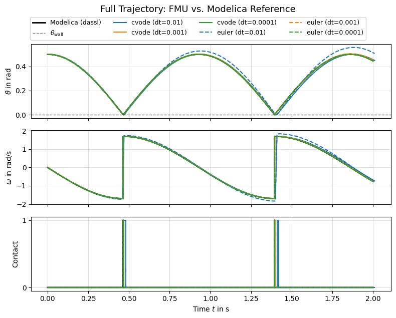
2.8.1. Full Trajectory Comparison#
The overview below shows the complete simulation window for all FMU configurations against the Modelica reference.
While the trajectories generally agree well between impacts, the accumulated timing errors after each contact lead to growing phase offsets — particularly visible for the coarser macro step sizes.
# --- Detect reference contact instants ---
t_ref_contact_vals = t_ref[np.where(contact_ref == 1)][::2]
t_contact_0 = t_ref_contact_vals[0]
t_contact_1 = t_ref_contact_vals[1]

print(f"Reference contact instants: t_0 = {t_contact_0:.6f} s, t_1 = {t_contact_1:.6f} s")
Reference contact instants: t_0 = 0.465078 s, t_1 = 1.395233 s
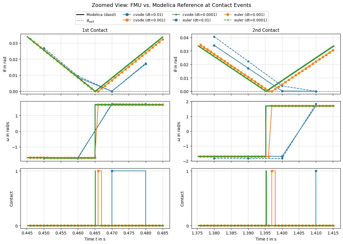
2.8.2. Zoomed View: Contact Events#
The plots below zoom into a narrow time window around each of the first two wall contacts.
Each column corresponds to one contact event. Within each column, the three rows show:
Position \(\theta(t)\): How closely the FMU trajectories track the Modelica reference near the wall.
Velocity \(\omega(t)\): The velocity reversal at impact — timing offsets are clearly visible here.
Contact flag: The discrete event signal; delayed detection in FMU co-simulation shifts the flag to the right.
The black reference curve is the direct Modelica dassl solution with tight tolerances and internal root-finding.
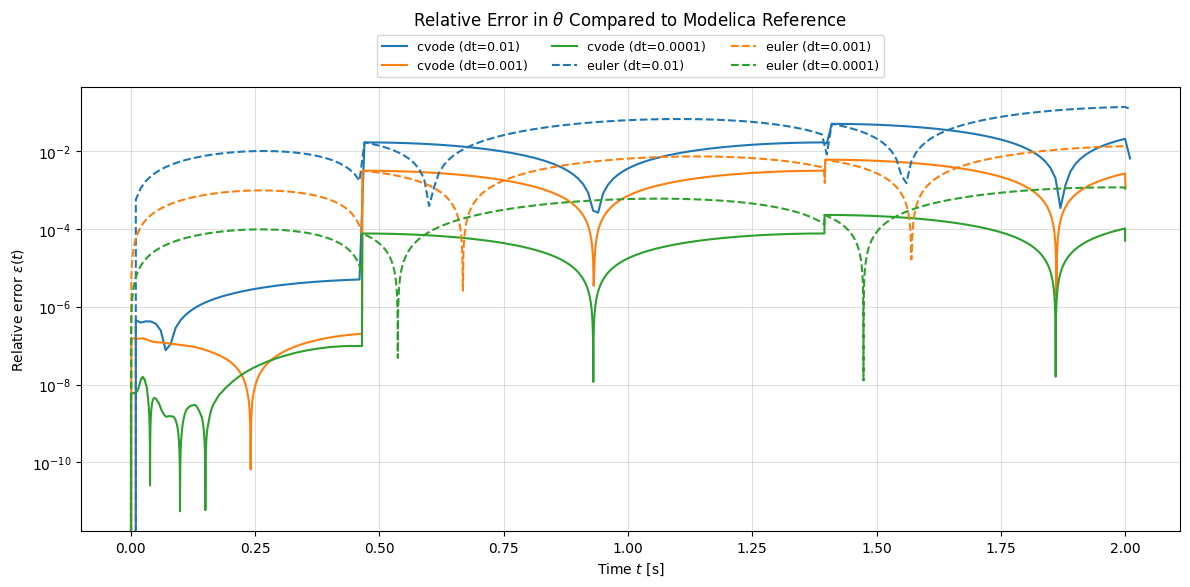
We calculate the relative error compared to the Modelica reference solution for theta:
2.9. Conclusion#
This tutorial showed that FMUs containing Modelica state events are sensitive to macro communication step size when used in co-simulation.
A smaller dt is typically required to detect impact events with high timing accuracy if no additional localization strategy is used.
In the following tutorials, we extend the FMUComponent workflow in syssimx with rollback and event-handling capabilities to localize events more accurately without relying only on globally small macro steps.